• Skip to main content
itrc_logo

Soil Background and Risk Assessment

Home
About ITRC
1 Introduction
1 Introduction
1.1 Audience
1.2 Purpose
1.3 Use of Background in the Risk Assessment Process
1.4 Limitations
2 Soil Background Definition 
2 Soil Background Definition
2.1 Natural Soil Background
2.2 Anthropogenic Ambient Soil Background
2.3 Additional Background Definitions
3 Establishing Soil Background
3.1 Introduction
3.2 Conducting a Soil Background Study
3.3 Choosing an Area for a Soil Background Study
3.4 Sampling
3.5 Laboratory Analysis
3.6 Using an Existing Soil Background Study
3.7 Background Dataset Analysis
3.8 Establishing Default or Site-Specific Soil Background
3.9 Extracting Site-Specific Background Dataset from an On-site Dataset
4 Using Soil Background in Risk Assessment
4.1 Representative Site Concentration to Compare to a BTV
4.2 Using Default Background
4.3 Using Site-Specific Background
4.4 Use of Background for Remedial Goals
4.5 Additional Considerations
5 Geochemical Evaluations
5.1 Geochemistry Is Not Statistics
5.2 Uses of Geochemical Evaluations
5.3 General Methodology
5.4 Nondetects
5.5 Key Geochemical Processes
5.6 Extracting Background Data from Existing Data
6 Using Geochemical Evaluations in Risk Assessment
6.1 Using Geochemical Evaluations During COPC Selection
6.2 Using Geochemical Evaluations During Risk Characterization
6.3 Considerations
7 Environmental Forensics Related to soil Background
7.1 Introduction
7.2 Polycyclic Aromatic Hydrocarbons
7.3 Total Petroleum Hydrocarbons (TPH)
7.4 Polychlorinated Biphenyls (PCBs)
7.5 Polychlorinated Dibenzo-p-Dioxins and Dibenzofurans (PCDD/F)
7.6 Perfluoroalkyl Substances (PFAS)
7.7 Remote Sensing
8 Conceptual Site Model and Data Quality Objectives
8.1 Conceptual Site Model
8.2 Data Quality Objectives
9 Sampling
9 Sampling
9.1 Background Reference Areas
9.2 Sample Depth
9.3 Sample Size
9.4 Sample Methods
9.5 Sampling Design
9.6 Sample Collection Methods
9.7 Sample Handling
10 Analytical Methods
10.1 Introduction
10.2 Obtaining Reliable Analytical Data
10.3 Analytical Limits
10.4 Sample Preparation
10.5 Analytical Test Methods
11 Statistics
11 Statistics
11.1 Data Requirements
11.2 Data Distribution
11.3 Treatment of Nondetects
11.4 Graphical displays
11.5 Outliers
11.6 Confidence Interval Limit, Coefficient, and Limit
11.7 Statistical Values Used to Represent Background
11.8 Statistical Tests to Compare Site and Background Datasets
11.9 Statistical Software
12 Regulatory Framework from State Survey
12.1 Description of State Survey
12.2 Overview of State Survey Results
12.3 State Survey Results
13 Existing Guidance and Studies
14 Case Studies
14 Case Studies
14.1 Minnesota Pollution Control Agency (MPCA) Soil Background Case Study
14.2 Former Firearms Training Range Soil Background Case Study
14.3 Region 4 RARE Urban Background Study
14.4 Geochemical Evaluation Case Study—Statistical Outlier is an Uncontaminated Soil Sample
14.5 Geochemical Evaluation Case Study—Statistical Outlier Is a Contaminated Soil Sample
14.6 Geochemical Evaluation Case Study–Contaminated Soil Sample Is Not a Statistical Outlier
14.7 Environmental Forensics Case Study—PAHs from Leaked Petroleum Versus Contaminated Fill
Frameworks
Frameworks
Framework 1
Framework 2
Framework 3
Appendices
Appendix A. Upper Limits Used to Estimate Background Threshold Values
Appendix B. Index Plots
Appendix C. Additional Sources of Information for PAHs in Soil
Additional Information
Team Contacts
Glossary
Acronyms
Acknowledgments
References
ITRC & EJ/DEI
Navigating this Website
Document Feedback


Soil Background and Risk Assessment
HOME

Appendix B. Index Plots

An index plot based upon a dataset, x1, x2, …, xn of size n represents a scatter plot obtained by plotting n pairs. An index plot represents a visual way of identifying intermediate and extreme outliers potentially present in a mixture on-site dataset. The data values need not be ordered in any way. The generation of index plots does not require any distributional assumptions and the availability of spatial data (x, y coordinates; latitude and longitude) associated with sampled locations. Since an index plot represents a scatter plot, any software equipped to generate a scatter plot can be used to generate an index plot.  

For clarity and usefulness of an index plot, one may want to order data by their population identification (ID) codes (for example, AOC1, AOC2…) (where AOC=area of concern) in the generation of an index plot as shown in Figure B1. On an index plot, observations from the various groups, including AOCs and an extracted background (for example, labeled as bk-extrct) data, are color-coded, where different colors represent different groups (AOCs). To avoid the distortion of the scale of an index plot, ND observations with elevated detection limits (DLs) may not be displayed on the index plot. An index plot can be formalized by drawing horizontal lines at one or more BTV estimates (for example, USL95, UTL 95-95), or at a prespecified regional cleanup level meant to compare individual on-site concentrations. The use of such index plots (Figures B1 and B2) comparing background (original or extracted) and the remaining on-site data (not included in extracted background data) may help the site managers in quickly identifying site AOCs and in making cleanup and remediation decisions at those AOCs.  

Figure B1 contains a color-coded index plot of the surface soil arsenic (prior to background extraction) dataset used in Section 3.9.5. It exhibits data of the AOCs and the existing background (labeled as bk) with a horizontal line displayed at a BTV estimate. Figure B2 has the similar index plot comparing the extracted background dataset (shown in blue) to the remaining contaminated AOCs concentrations. 

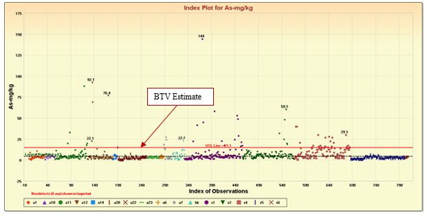
Horizontal line displayed at the BTV estimate =15.1 mg/kg.

Figure B1. Index plot comparing surface soil arsenic concentrations of the existing background (bk) and various AOCs (prior to background extraction). 

Source: Anita Singh, ADI-NV Inc. 

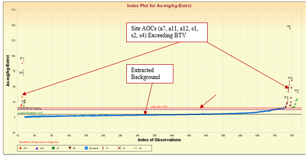
Horizontal lines displayed at the BTV estimate, 15.1 mg/kg, and the largest nondetect value, 4.5 mg/kg.

Figure B2. Index plot comparing surface soil arsenic concentrations of the extracted background (bk-extrct) and the remaining AOCs (not included in bk-extrct). 

Source: Anita Singh, ADI-NV Inc. 

image_pdfPrint this page/section
glossary Full PDF
glossaryGlossary
referencesReferences
acronymsAcronyms
ITRC
Contact Us
About ITRC
social media iconsClick here to visit ITRC on FacebookClick here to visit ITRC on TwitterClick here to visit ITRC on LinkedInITRC on Social Media
about_itrc
Permission is granted to refer to or quote from this publication with the customary acknowledgment of the source (see suggested citation and disclaimer). This web site is owned by ITRC • 1250 H Street, NW • Suite 850 • Washington, DC 20005 • (202) 266-4933 • Email: [email protected] • Terms of Service, Privacy Policy, and Usage Policy ITRC is sponsored by the Environmental Council of the States.