14 Case Studies
14.1 Minnesota Pollution Control Agency (MPCA) Soil Background Case Study
This case study presents an example of a state regulatory agency establishing statewide default natural soil background values using data from an existing soil natural background study. The MPCA established their first set of statewide soil background values using the U.S. Geological Survey’s (USGS) Geochemical and Mineralogical Data for Soils of the conterminous United States ((MPCA 2016), (Smith et al. 2013)). The objective of USGS’s study was to sample for natural soil background, avoiding anthropogenic sources.
Soil screening values used to evaluate cleanup sites are generally derived by state regulatory agencies using the USEPA methodology (USEPA 1996), toxicity values, exposure parameters, and chemical-specific information. These values are purely risk based, intended to protect human health or the environment, and do not take natural soil background into consideration. MPCA’s soil screening values are called soil reference values (SRVs). When MPCA revised their SRVs to incorporate more recent toxicity and exposure parameters, they recognized that eight of the revised SRVs for inorganics could potentially be below natural background concentrations in soil. Those eight inorganics were aluminum, arsenic, barium, chromium, cobalt, iron, thallium, and vanadium. This case study describes the process MPCA used to determine whether the SRVs were below natural soil background concentrations and, if so, derive default soil background threshold values (BTVs).
14.1.1 Existing data
Since funding could not be obtained for MPCA to conduct a statewide soil background study, the agency evaluated existing studies that could be used to determine statewide background concentrations for the inorganics of interest.
A report by the Minnesota Geological Survey (Thorleifson et al. 2007) was considered, but the purpose of obtaining that data was for mineral exploration rather than to determine natural background concentrations of inorganics. Samples were obtained from areas thought to have higher concentrations of minerals rather than areas that were not impacted by anthropogenic sources. In addition, the study included both soil and sediment data that would not be easy to identify and separate (Thorleifson et al. 2007).
Two studies often used to determine soil background concentrations of metals, the USGS Boerngen and Shacklette studies ((Boerngen and Shacklette 1981), (Shacklette and Boerngen 1984)), were considered. These studies include concentrations of metals and other trace elements in soil of the conterminous United States, with samples collected in the 1960s and 1970s. However, the USGS more recently conducted a national-scale geochemical and mineralogical survey of soils of the conterminous United States from 2007 to 2013 ((Smith et al. 2013) and (Smith et al. 2014)).
USGS Soil Geochemical and Mineralogical Background Study
The most recent and comprehensive U.S. soil geochemical and mineralogical background study was conducted by the USGS from 2007 to 2013. The USGS developed protocols, performed pilot studies, and collected soil samples across the conterminous United States to determine natural background concentrations for constituents, including inorganics (Smith et al. 2013). Sites were selected to represent a spatially balanced density of approximately one site per 1,600 km2 from areas unlikely to be contaminated. In total, 14,434 samples from nearly 5,000 sites were collected across the United States. Samples at each site included a surface sample collected from 0 to 5 centimeters, a composite of the soil A horizon, and a deeper sample called the soil C horizon, not exceeding a depth of approximately 80–100 cm.
Samples were prepared for analyses using standard USGS analytical protocols, which included air drying at ambient temperatures, sieving to less than 2 mm, followed by grinding to less than 150 µm. Prepared samples were aggressively digested using a four-acid mixture (hydrochloric, nitric, hydrofluoric, and perchloric) heated to temperatures between 125 and 150°C. This digestion method dissolves most silicate, sulfide, oxide, and carbonate minerals. Total element concentrations for 41 elements were measured by inductively coupled plasma-atomic emission spectrometry (ICP-AES) and by inductively coupled plasma-mass spectrometry (ICP-MS). Mercury, selenium, and arsenic were analyzed by single-element analytical methods. Organic carbon concentrations for the 0 to 5 cm soil and soil A horizon were calculated from the difference between analyzed inorganic carbon and total carbon. Mineralogy was determined for splits of the soil A and C horizons by a quantitative X-ray diffraction method. Smith et al. (2013) provides details of sample site selection and analytical methods, as well as all geochemical and mineralogical data. Interpolated maps displaying the data are available in Smith et al. (2014) and were also integrated into an interactive website (Smith et al. 2019).
USEPA methods (SW846 3050B or 3051A) used at cleanup sites are similar to analytical methods used by the USGS, but distinctions are evident for preparation methods and, particularly, for sample digestion. The USEPA method includes sample homogenization, but it is up to each individual lab to decide how to do this. USEPA methods also use a less aggressive aqua regia digestion, although there can be differences for digestion of some inorganics. Since USEPA digestions are not intended to yield total or near-total values, geochemical results are not directly comparable to results obtained using USGS’s analytical methods. It is likely that concentrations determined for the same soil sample using the more aggressive USGS methods will generally be higher than concentrations determined by USEPA’s methods. This, however, may not always be the case and will vary depending on specific inorganic constituents as well as local geology. Sample mineralogy also may influence the effectiveness of the two digestion methods. Overall, inconsistencies between the results of each analytical approach are due to the differences in preparation and digestion methods, and caution must be used when comparing data
MPCA chose to use this more recent USGS survey of soils to establish state background values. Soil from a total of 137 sites was collected in Minnesota as part of this study. Laboratory analysis of the soil samples was completed in 2013. USGS took the following measures to ensure samples were not collected from areas impacted by anthropogenic sources: no samples were collected within 200 m of a major highway, within 50 m of a rural road, within 100 m of a building or structure, or within 5 km downwind of active major industrial activities such as power plants or smelters. Samples at each site were obtained from three different intervals below the ground surface: 0 to 5 cm, A horizon, and C horizon (Smith et al. 2013). Splits of all samples collected by the USGS are currently stored in a sample archive in Denver, Colorado.
14.1.2 USGS and USEPA analytical methods
Soil preparation and analytical methods used by the USGS differ from the USEPA methods typically used for cleanup sites in state and federal remediation programs. Differences in concentrations resulting from the two methods depend on the geological characteristics of the area where the sample was taken, and also on the chemical nature of each analyte. As a result, concentrations obtained using these two methods are not generally comparable.
Sample preparation using the USGS method begins with air drying at ambient temperature, sieving to less than 2 mm and grinding to less than 150 μm. The USEPA method (SW846 3050B or 3051A) begins with suggested sample homogenization but leaves the final decision on how to prepare an individual sample up to the laboratory. A consequence is that the USGS preparation method results in finer grained samples compared to samples prepared using USEPA’s method, thus leading to more surface area available for digestion.
In addition, a near-total four-acid digestion is used in the USGS method. Sieved and ground samples are digested with a mixture of hot nitric, hydrochloric, hydrofluoric, and perchloric acid. Samples for arsenic analyses are first fused in a mixture of sodium peroxide and sodium hydroxide and then dissolved in hydrochloric acid. The USEPA method uses a less aggressive aqua regia digestion. For arsenic and thallium analyses, digestion is accomplished using hydrogen peroxide and nitric and hydrochloric acid. Digestion for the other inorganics is accomplished using hydrogen peroxide and nitric acid.
Methods of detection used for the eight inorganics in the USGS analytical method are:
- inductively coupled plasma–atomic emission spectrometry (ICP-AES) for aluminum, chromium, iron, and vanadium
- ICP-MS for cobalt and thallium
- hydride-generation atomic absorption spectrometry for arsenic
Methods of detection used for the eight inorganics using the USEPA analytical method are:
- inductively coupled plasma–atomic emission spectrometry (ICP-AES) for aluminum, barium, chromium, cobalt, iron, and vanadium
- ICP-MS for arsenic and thallium
The key distinctions between USGS and USEPAs analytical methods are:
- The USGS preparation method results in more surface area available to be digested, whereas the USEPA preparation method does not require a specific procedure and may result in less surface area available for digestion.
- The USGS digestion is intended to result in a true total concentration of all metals in the soil sample, while USEPA’s digestion is not intended to be a total digestion and thus results in lower metals concentrations of some inorganics in the soil sample.
In most cases the USGS method results in higher concentrations than the USEPA method. In these cases, soil background values based on the USGS data would be higher than those based on USEPA’s method. Since USEPA’s method is used to characterize site concentrations at cleanup sites, this would result in an inappropriate comparison. Higher site concentrations would be incorrectly characterized as being representative of background since USGSs background value would be higher than if the sample were analyzed using USEPA’s method.
14.1.3 USEPA method reanalysis
Since it was not appropriate to directly use USGS’s data to establish a soil background value for a cleanup site, MPCA reanalyzed a subset of USGS soil samples using the USEPA’s method to evaluate the differences in results between the two methods.
The archived USGS soil samples were outside of their holding time when they were reanalyzed for the MPCA study. Samples had been stored at the USGS Denver, Colorado, facility at room temperature since collection. Although the longer than normal storage time under room temperature conditions is not expected to significantly impact the results of the analyses of the eight specific inorganics that were reanalyzed, this has not been confirmed by laboratory testing.
MPCA could not reanalyze more than one sample depth due to cost constraints. Even though human and ecological receptors could be exposed to both the 0 to 5 cm below the ground surface and A horizon, MPCA chose to reanalyze the 0 to 5 cm depth based on the following rationale:
- The 0 to 5 cm depth was most relevant to human receptor exposure.
- Results from the 0 to 5 cm and the A horizon appeared to be similar.
A subset of 48 USGS 0 to 5 cm depth soil samples (out of 137 total available Minnesota samples) was chosen to be reanalyzed using the USEPA method. Samples were selected based on the following factors:
- 24 samples were chosen in a stratified random fashion to represent differences in geology across the state. This was accomplished by choosing samples with varying abundances of quartz and clay, as proportions of these two silicate minerals are a good proxy for soil parent materials.
- 14 samples were chosen in a stratified random fashion to represent the different major land resource areas and land cover across the state, which incorporated variations in vegetation and climate.
- 10 nonrandom samples were chosen based on their proximity to major cities and the Minnesota River to capture areas with potentially higher populations. They were not chosen to capture anthropogenic ambient soil background; the USGS study was aimed at collecting natural soil background.
Three of the archived samples originally chosen for reanalysis using USEPA methods could not be located in the USGS archive so they were not analyzed (two chosen based on differences in geology and one chosen based on proximity to major cities and the Minnesota River). A total of 45 USGS samples were reanalyzed using USEPA’s soil analytical method. Thirty-six of these were chosen in a stratified random fashion, and nine were chosen based on their proximity to major cities and the Minnesota River. Randomly chosen datasets are recommended to be used when performing statistical calculations.
Samples were analyzed using USEPA Method 6010C (ICP-AES) for aluminum, barium, chromium, cobalt, iron, and vanadium and USEPA Method 6020A (ICP-MS) for arsenic and thallium.
14.1.4 Statistics
USEPA’s ProUCL software and associated technical guide were used to evaluate for potential outliers, determine dataset distributions, and calculate a soil background value (BTV) from the Minnesota sample subset of the USGS study data (USEPA 2013).
Outliers were determined using the Rosner outlier test and further evaluated using Q-Q plots, histograms, and box plots generated using ProUCL, version 5.0. BTV calculations were performed both with and without outliers using ProUCL’s “Upper Limit-BTVs” module.
ProUCL’ s “Upper Limit-BTVs” calculation was used to determine the BTV for each inorganic. This ProUCL function can be used for datasets with or without nondetect data. It determines whether the dataset is parametric (fits a normal, gamma, or lognormal distribution) or nonparametric and provides the following types of BTVs:
- upper percentiles
- upper prediction limits (UPL)
- upper simultaneous limit (USL)
- upper tolerance limit (UTL)
According to USEPA’s ProUCL guidance, upper percentiles and UPLs are not appropriate to use when establishing a default soil BTV where there will be a large number of comparisons to the BTV (expected for statewide default values). Using UPLs, which are designed to minimize false positives, will in this case actually result in high false positive error rates, meaning a larger number of soil concentrations reflecting real background levels would exceed the BTV and appear as if they are contaminated. Another concern with the UPL is that it is calculated based on an expected number of future samples. With a statewide dataset, it is unknown how many future samples will be compared to the BTV.
USLs are also not appropriate to use when establishing a default BTV where there will be a large number of comparisons to the BTV (expected for statewide default values). A USL represents an upper limit on the largest value of the dataset and would result in high false negative error rates, meaning a large number of soil concentrations that represent actual contamination would not exceed the BTV and appear to represent background levels.
UTLs were chosen to establish the BTVs because they are appropriate to use when establishing a default BTV where there will be a large number of comparisons to the BTV (expected for statewide default values). Using UTLs is not likely to result in large false positive or false negative error rates. MPCA chose to calculate 95-95 UTL representing the 95% upper confidence limit on the 95th percentile.
14.1.5 Results
Differences in results from the USGS and USEPA’s analytical methods varied widely among the inorganics. For some parameters the differences were very little, but for others they were significant.
MPCA investigated the possibility of using the USEPA method by reanalyzing 45 samples to establish soil BTVs. Since the 45 samples that were reanalyzed using the USEPA method were not all chosen randomly (only 36 were), a comparison was performed between the random (36 samples) and nonrandom (45 samples) datasets to determine whether they were similar. MPCA compared the distributions, graphical displays, and outliers of the five datasets listed below using USEPA’s ProUCL.
- USGS method analyzed 137 samples (all samples from Minnesota)
- USGS method analyzed 45 samples (subset including nine nonrandom data points)
- USEPA method reanalyzed 45 samples (subset including nine nonrandom data points)
- USGS method analyzed 36 samples (subset of only randomly selected data points)
- USEPA method reanalyzed 36 samples (subset of only randomly selected data points)
Since these datasets appeared to be similar, MPCA determined that it was appropriate to derive BTVs based on the results of the USEPA method reanalyzed subset of 45 samples despite the fact that only 36 were chosen randomly.
The datasets were evaluated using USEPA’s ProUCL with and without outlier removal to determine the following:
- BTVs using the complete 137 sample USGS analyzed dataset for Minnesota
- BTVs using the results of the 45 samples reanalyzed using USEPA methods
Minnesota-specific maps of inorganic concentrations similar to those USGS created for the United States were also created. These maps can be used by risk assessors and project managers on a site-specific basis since the maps show the difference in concentrations across the state of Minnesota. Soil background concentrations of inorganics are heterogeneous. Although a range more accurately describes soil background, one value is often selected due to program needs.
BTVs and the percent difference from the results from the reanalysis using the USEPA analytical method on the 45 samples compared to results from the USGS analytical method using the 137 samples are shown in Table 14‑1. This comparison included descriptive statistics and graphical displays. There was very little difference in the results of the two methods for arsenic. The BTV using the entire 137-sample USGS-analyzed dataset and the 45-sample USEPA-reanalyzed dataset was identical (9 mg/kg). Cobalt results were also similar, with the BTVs calculated from the two datasets having an 8% difference. Differences between the aluminum (68%), barium (70%), and chromium (62%) BTVs were much more significant. A BTV for thallium could not be calculated due to the number of nondetects in the dataset. In six cases the BTV was greater than the SRVs. In those cases, the BTV replaced the SRV (MPCA 2016a (MPCA 2016)).
Table 14‑1. USEPA analytical method results
| Inorganic | MPCA Residential SRV (mg/kg) | USGS BTV (UTL) of 137 Original Samples—USGS Analytical Method (mg/kg) | USEPA BTV (UTL) of 45 Reanalyzed Samples—USEPA Analytical Method (mg/kg) | Percent Difference USEPA and USGS BTVs |
| Aluminum | 15,000 | 60,000 | 19,000 | -68% |
| Arsenic | 0.051 | 9 | 9 | 0% |
| Barium | 3,000 | 710 | 210 | -70% |
| Chromium | 23,000 (III) 11 (VI) |
71 | 27 | -62% |
| Cobalt | 4.6 | 13 | 12 | -8% |
| Iron | 11,000 | 38,000 | 29,000 | -24% |
| Thallium | 0.15 | None | 0.29 | NA |
| Vanadium | 1.1 | 119 | 62 | -48% |
|
Bold, shaded values highlight background concentrations above MPCA SRVs. All BTVs are 95-95 UTL, representing the 95% upper confidence limit on the 95th percentile. Percent difference USEPA and USGS BTVS defined as (((USEPA BTV – USGS BTV)/USGS BTV))*100) |
||||
14.2 Former Firearms Training Range Soil Background Case Study
This site is a former firearms training range used for small firearms training. The COPC associated with historical firearms training activities at the Site identified during environmental investigations included antimony, arsenic, and lead. Remedial soil excavation activities were conducted in 2020. Following the soil excavation activities, only elevated soil concentrations of arsenic were detected in the confirmation samples.
This study presents an example of establishing a soil background level higher than the regulatory default ambient arsenic screening level of 12 mg/kg used as a cleanup goal for arsenic at the Site.
14.2.1 Development of a site-specific arsenic cleanup goal
The removal action confirmation sample results included only the post-removal soil confirmation samples from the margins of the remedial excavation and not the complete soil dataset prior to the soil removal action. Figure 14‑1 presents the probability plot of the 30 soil samples.
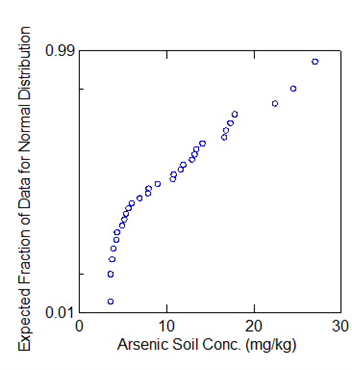
Figure 14‑1. Probability plot of 30 samples.
Figure 14‑2 summarizes the confirmation dataset in a box and whisker plot.
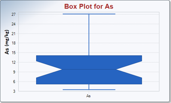
Figure 14‑2. Box and whisker plot of confirmation data.
As can be seen from these two plots, the majority of arsenic concentrations are between 5 mg/kg and 14 mg/kg.
Ninety-eight soil samples were analyzed for metals at a nearby active firearms training range. Arsenic concentrations in soil ranged from 0.62 mg/kg to 21 mg/kg. Only four samples exceeded 12 mg/kg, specifically 13, 14, 16, and 21 mg/kg. Six off-site background samples were also collected. Off-site arsenic concentrations ranged from 4.2 mg/kg to 7.0 mg/kg.
For the Site, the two highest concentrations, 24.5 and 27 mg/kg, were removed as potential outliers based on multiple lines of evidence, including 1) graphical evaluation based on probability and box plots; 2) outlier removal based on ProUCL; and 3) arsenic data from a nearby site. Ultimately, professional judgment was used in evaluating the multiple lines of evidence and selecting the final dataset. The Site arsenic dataset was evaluated using the USEPA ProUCL, version 5.1, statistical software. Specifically, the descriptive statistics and BTVs were evaluated for the Site dataset. The ProUCL outputs included general statistics, goodness of fit, and estimated upper tolerance limits (background threshold values). Given the small sample size—only 30 arsenic samples—the 90th- or 95th-percentile estimates were selected as the more appropriate estimators of an upper-bound arsenic background value. Based on the ProUCL outputs, the data may be either approximate normal or lognormal in terms of the data distribution.
Assuming a normal distribution, the 90th- and 95th-percentile arsenic concentrations were 16.5 and 18.4 mg/kg, respectively. Assuming a lognormal distribution, the 90th- and 95th-percentile arsenic concentrations were 17.4 and 21.4 mg/kg, respectively. The nonparametric analysis, which does not assume any specific data distribution, resulted in 90th- and 95th-percentile arsenic concentrations of 17.0 and 17.6 mg/kg, respectively.
14.2.2 Recommendations
Given the small sample size and no discernible distribution of the arsenic dataset, the nonparametric 95th-percentile arsenic concentration of 18 mg/kg was selected as the most appropriate upper bound arsenic screening level for the site. This value is also consistent with (1) the site-specific off-site background data collected, where the maximum arsenic concentration was 18.3 mg/kg, and (2) the arsenic data from the nearby site.
14.3 Region 4 RARE Urban Background Study
In 2017, USEPA Region 4 was awarded a Regional Applied Research Efforts (RARE) Grant to work in collaboration with USEPA Office of Research and Development and southeastern regional states to develop a robust dataset to characterize contaminants present in urban soils deriving from natural and anthropogenic background, unrelated to chemical spills or industrial waste. A sampling and analysis plan (SAP) and a quality assurance project plan (QAPP) were developed and applied to eight cities within Region 4. The SAP and QAPP for the project were developed to ensure data collected would be defensible and reproducible. Soils were analyzed for RCRA 8 metals and PAHs.
14.3.1 Sample Design
A 7-mile by 7-mile grid was applied over each city center and divided into ½-mile by ½-mile grids, totaling 196 cells per city. Using a random number generator, 50 cells were selected for sample collection. Sample location criteria required soils to be representative of an urban setting, undisturbed by recent activity, not potentially impacted by nearby industry, and in public areas such as rights-of-way. Sample locations not acceptable included private/residential yards, industrial properties, areas of recent development, and low-lying areas subject to flooding or inundation. Samples were collected within the selected grid that met the criteria. If no areas within a sample grid met the criteria, then the next randomly selected grid was chosen.
A discrete sample was collected at each location using a turf profiler. The turf profiler sampling tool was modified to be 8.9 cm (3.5 in) wide, 2.5 cm (1 in) thick, and 10.2 cm (4 in) deep. The top 5 cm (2 in) of soil were retained for analysis with top organic material and remaining soils discarded.
Each sample was mixed and rigorously subsampled in the field. Samples designated for PAH analysis were sent in 4-ounce amber jars to an USEPA Contract Laboratory Program laboratory. Samples designated for metals analysis were sent in 4-ounce Whirl-Paks to USEPA’s Las Vegas lab to be dried, sieved, and prepared for analysis. Once prepared, samples were shipped to USEPA Region 4 Science and Ecosystem Support Division (SESD) laboratory for analysis. Soil samples were analyzed for metals using USEPA Method 6010C and PAHs using USEPA Method 8270D. Three equipment blanks and three field blanks were collected per city.
14.3.2 Results
Metals analysis included arsenic, barium, cadmium, chromium, lead, mercury, selenium, and silver. Summary statistics were compiled for each contaminant by city and calculated using USEPA ProUCL software. The full dataset of metals and PAHs can be found at the USEPA Regional Urban Background Study website. Selected data are summarized below.
Mean arsenic concentrations in seven of the eight cities were above the USEPA regional screening level (RSL) of 0.68 mg/kg. The mean concentrations ranged from 0.55 mg/kg to 19.71 mg/kg. Noting that anthropogenic background of arsenic in some cities is above USEPA’s RSL can be useful not only in determining whether the presence of arsenic in a given location is site-related contamination but in developing appropriate cleanup goals and guiding risk assessment.
Mean lead results in all eight cities were less than the current USEPA screening level of 400 mg/kg. Mean lead concentrations ranged from 15.06 mg/kg to 216.1 mg/kg. Summary statistics for lead are shown in Table 14‑2. Box and whisker plots for lead are shown by city in Figure 14‑3.
Table 14‑2. Lead summary statistics
| City | Num Obs | Minimum | Maximum | Mean | Geo-Mean | SD |
| Chattanooga | 50 | 14 | 580 | 96.22 | 60.1 | 122 |
| Columbia | 50 | 1.7 | 200 | 40.79 | 25.58 | 38.41 |
| Gainesville | 50 | 2 | 110 | 15.06 | 9.187 | 18.62 |
| Lexington | 50 | 18 | 420 | 81.51 | 56.33 | 88.63 |
| Louisville | 50 | 25 | 1100 | 155.7 | 99.24 | 192.3 |
| Memphis | 50 | 13 | 1000 | 121 | 63.43 | 201.7 |
| Raleigh | 50 | 7.6 | 180 | 33.84 | 22.72 | 37.1 |
| Winston-Salem | 50 | 20 | 1400 | 216.1 | 128.8 | 247.2 |
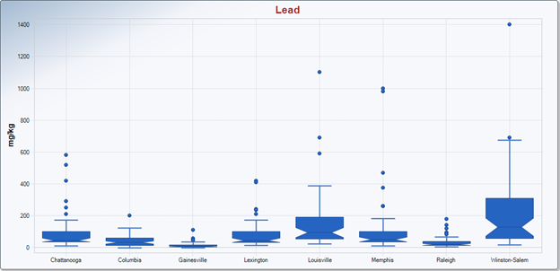
Figure 14‑3. Box and whisker plots for lead.
14.3.3 Uses of Methods and Data
The robust dataset collected throughout the southeastern states could be used in developing cleanup goals, assessing risk, evaluating sample results, designing remedies, and evaluating the impact of natural disasters. The Region 4 Urban Background Study results highlight the difference in natural versus anthropogenic background. It is important to establish the difference between background concentrations and elevated contamination due to a spill or release in a particular area.
The methodology has been used by other USEPA regions along with universities to develop their own dataset of urban background soils. The data collected in Region 4 have been used at multiple sites and by two universities. The methods are easily adaptable to fit the area one would test for urban background, as was done for the City of Chattanooga.
The Urban Background Study Sampling and Analysis Plan and Quality Assurance Project Plan is publicly available: (https://www.epa.gov/research-states/regional-urban-background-study-webinar-archive).
The background dataset is also publicly available: https://www.epa.gov/risk/regional-urban-background-study.
14.4 Geochemical Evaluation Case Study—Statistical Outlier is an Uncontaminated Soil Sample
This case study involves a former military munitions site located in mountainous terrain in Colorado. A total of 12 candidate background subsurface soil samples (limited number due to budget constraints) were collected from an undeveloped adjacent property hydraulically upgradient of a former military munitions site that had soils geologically similar to the site. The discrete samples were collected from 0.3 to 0.5 m below ground surface and analyzed for metals; these results formed a candidate subsurface soil background dataset.
Dixon’s statistical outlier test was performed for every trace element of interest for this site, including vanadium (a description of Dixon’s test is provided in Table 11‑2 in Section 11.5). The maximum vanadium (V) concentration (51.1 mg/kg) failed Dixon’s outlier test at a significance level (α) of 0.05. Geochemical evaluation was performed to determine whether the elevated vanadium concentration was due to contamination or just inherent variability in soil concentrations. First, soil descriptions in the soil boring logs were studied, along with historical aerial photographs and site history, to identify possible sources for the elevated vanadium at that location; no sources were found. The sample with the outlier concentration was collected near an unpaved forest road, distant from the site.
As discussed in Section 5.3, the next step was to evaluate the concentrations of aluminum versus iron, because they are qualitative grain-size indicators, as well as primary reference elements (Figure 14‑4). The concentrations of iron and aluminum covary (as the concentration of iron increases, the concentration of aluminum increases) and the samples exhibit similar Al/Fe ratios, indicating there is no aluminum or iron contamination in any of the candidate background samples. This confirms that these elements can serve as reference elements for the evaluation of trace elements of concern. The samples with higher aluminum and iron concentrations have more fine-grained minerals (such as clays and iron oxides), so they are expected to have naturally higher trace element concentrations.
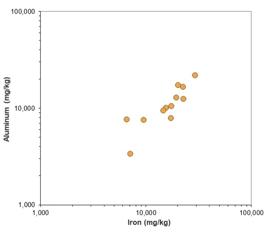
Figure 14‑4. Scatter plot of aluminum versus iron for background subsurface soil.
Source: Karen Thorbjornsen, APTIM.
Scatter plots were prepared of vanadium versus aluminum (not depicted here, since the vanadium concentrations did not covary with aluminum concentrations in the scatter plot for this dataset) and vanadium versus iron (Figure 14‑5). As discussed in Section 5.5.2, vanadium has a strong affinity for adsorption on iron oxide minerals in soil (Kabata-Pendias 2010). Vanadium was observed to covary with iron (Figure 14‑5). The sample with the highest vanadium concentration also had the highest iron concentration (29,500 mg/kg).
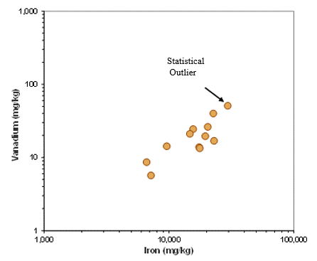
Figure 14‑5. Scatter plot of vanadium versus iron for background subsurface soil.
Source: Karen Thorbjornsen, APTIM.
In addition to the scatter plot (Figure 14‑5), a ratio plot (Figure 14‑6) of vanadium concentrations versus V/Fe ratios was prepared.
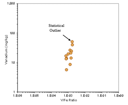
Figure 14‑6. Ratio plot of vanadium versus V/Fe for background subsurface soil.
Source: Karen Thorbjornsen, APTIM.
In Figure 14‑5, all the background samples (including the statistical outlier) form a common trend with a positive slope. In Figure 14‑6, all samples (including the statistical outlier) have similar V/Fe ratios. This evaluation indicates the elevated vanadium concentration is due to preferential enrichment of iron oxide minerals in soil at that location and is not due to contamination by vanadium. Thus, the maximum vanadium concentration (the statistical outlier) was retained in the candidate subsurface soil background dataset.
14.5 Geochemical Evaluation Case Study—Statistical Outlier Is a Contaminated Soil Sample
Twenty-nine candidate background subsurface soil samples were collected from an undeveloped and heavily wooded property adjacent to (but hydraulically upgradient of) a former military facility located in glacial terrain in New Hampshire, with similar soils as the site. The discrete samples were collected from 0.5 to 0.6 m feet below ground surface and analyzed for metals; these results then formed a candidate subsurface soil background dataset.
Rosner’s statistical outlier test was performed for every trace element of interest for this site, which included arsenic (a description of Rosner’s test is provided in Table 11‑2 in Section 11.5). The maximum arsenic (As) concentration in subsurface soil (61.4 mg/kg) failed Rosner’s outlier test at a significance level (α) of 0.05. Geochemical evaluation was performed to determine whether this elevated arsenic concentration is due to arsenic contamination of this soil sample or if it is due to inherent variability in soil concentrations. Review of the soil description and the physical setting for that sample location revealed nothing unusual that would indicate a site-related arsenic contaminant source.
Aluminum and iron concentrations covary for this dataset (see scatter plot in Figure 14‑7) and the samples have similar Al/Fe ratios. This indicates there is no aluminum or iron contamination in the candidate background samples and confirms that the two elements can serve as reference elements for the evaluation of trace elements of concern.
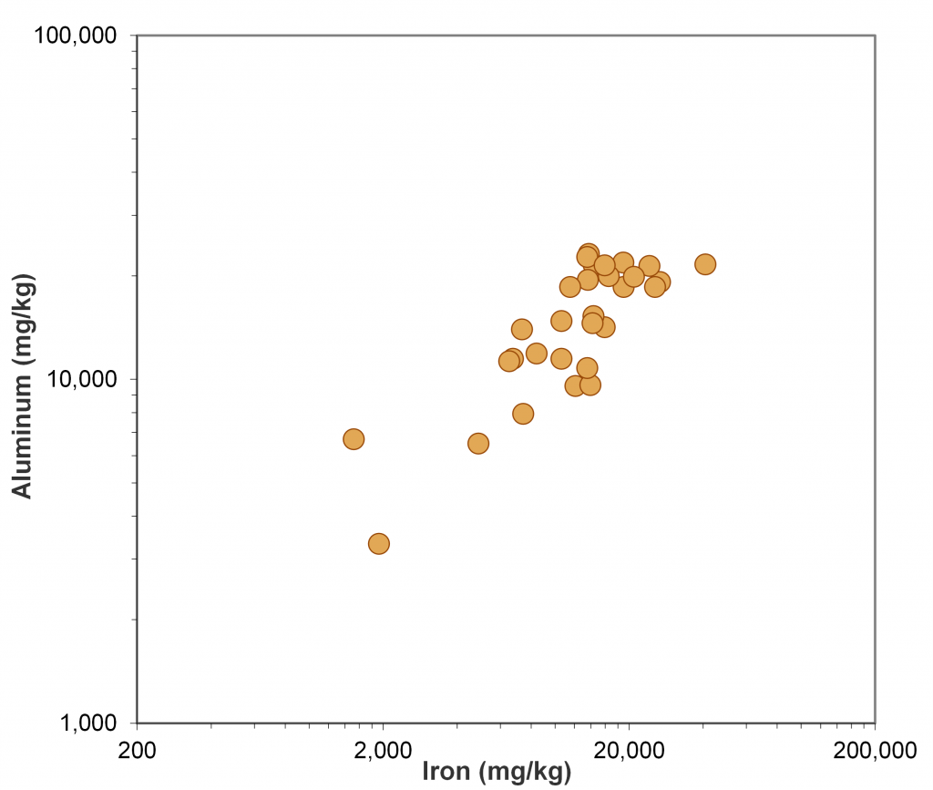
Figure 14‑7. Scatter plot of aluminum versus iron for background subsurface soil.
Source: Karen Thorbjornsen, APTIM.
As discussed in Section 5.5.2, arsenic has a strong affinity to adsorb on iron oxide minerals in soil ((Bowell 1994), (Kabata-Pendias 2010), so the arsenic and iron concentrations are expected to covary in soil samples in the absence of arsenic contamination. In the scatter plot of arsenic versus iron concentrations (Figure 14‑8), all but one of the samples lie along the same trend, reflecting the natural association of arsenic with iron oxides in soil. The sample with the statistical outlier concentration lies above and to the left of the trend. Although it has the highest arsenic, it has relatively low iron (as well as relatively low concentrations of the other major elements).
Figure 14‑8. Scatter plot of arsenic versus iron for background subsurface soil.
Source: Karen Thorbjornsen, APTIM.
In the ratio plot in Figure 14‑9, all samples (except the statistical outlier) have similar As/Fe ratios; the statistical outlier has a higher As/Fe ratio relative to the other 28 subsurface soil samples. The arsenic concentration in this sample is anomalously high, likely due to contamination of the sample by arsenic. Thus, this concentration was excluded from the candidate background dataset for arsenic, leaving this dataset with 28 arsenic concentrations.
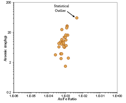
Figure 14‑9. Ratio plot of arsenic versus As/Fe for background subsurface soil.
Source: Karen Thorbjornsen, APTIM.
For arsenic at this site, geochemical evaluation confirmed the result of the statistical outlier test.
14.6 Geochemical Evaluation Case Study–Contaminated Soil Sample Is Not a Statistical Outlier
A total of 10 candidate background surface soil samples (limited number due to budget constraints) were collected from a portion of a former military munitions site located in Wyoming that had never been developed and was hydraulically upgradient of the area of interest. The background soils were geologically similar to those in the area of interest. The discrete surface soil samples were collected from 0 to 5 cm below ground surface and analyzed for metals; these results then formed a candidate background dataset.
Dixon’s statistical outlier test was performed for every trace element of interest for this site, which included lead (a description of Dixon’s test is provided in Table 11‑2 in Section 11.5). The maximum lead (Pb) concentration in subsurface soil (17.4 mg/kg) passed Dixon’s outlier test at a significance level (α) of 0.05. From visual inspection this concentration appeared to be higher than the other lead concentrations, so a geochemical evaluation was performed to double-check whether the concentration was elevated due to lead contamination of soil at that location or just due to inherent variability in soil concentrations.
Review of the soil description for that sample location revealed nothing unusual that would indicate a site-related lead contaminant source; the sampled soils were the same silty sand as noted for the other background sample locations. The aluminum and iron concentrations covary (see scatter plot in Figure 14‑10) and the samples have similar Al/Fe ratios, indicating that there is no aluminum or iron contamination in the candidate background samples and confirming that the two elements can serve as reference elements.
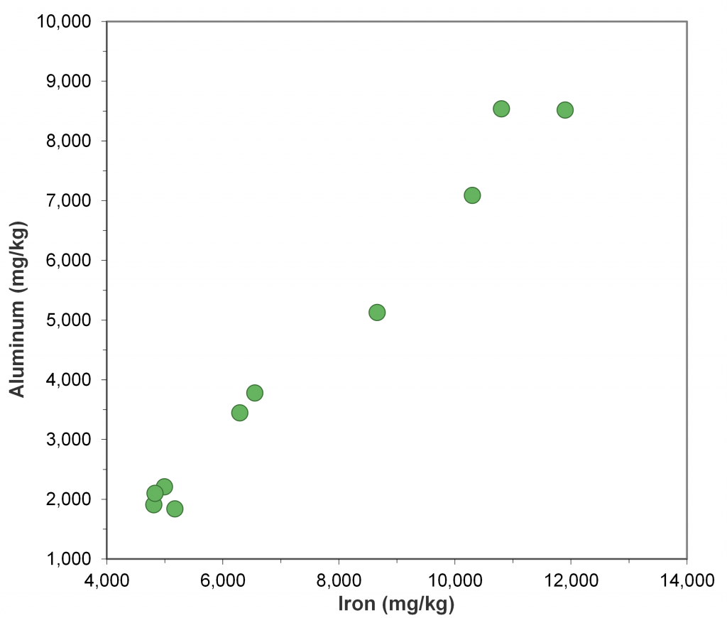
Figure 14‑10. Scatter plot of aluminum versus iron for background surface soil.
Source: Karen Thorbjornsen, APTIM.
Although lead can adsorb on iron oxides and manganese oxides, it also has a strong affinity to adsorb on clay minerals in soil ((McLean and Bledsoe 1992), (Kabata-Pendias 2010)). A scatter plot of lead versus aluminum (Figure 14‑11) and corresponding ratio plot (Figure 14‑12) were prepared.
In Figure 14‑11, all but one of the background samples lie along a common trend; the sample with the maximum lead concentration has one of the lowest aluminum concentrations and lies above the trend. This sample also has low concentrations of the other major elements.
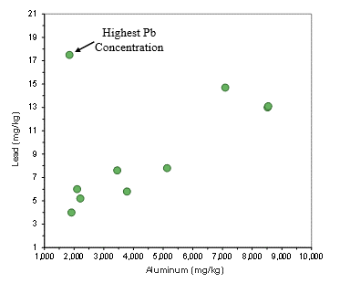
Figure 14‑11. Scatter plot of lead versus aluminum for background surface soil.
Source: Karen Thorbjornsen, APTIM.
In Figure 14‑12, most samples have similar Pb/Al ratios; the sample with the maximum lead concentration has a higher Pb/Al ratio than the other nine surface soil samples. Geochemical evaluation indicates the maximum lead concentration is anomalously high (likely due to lead contamination of the sample and suspected to be munitions-related) and is not naturally elevated, even though this data point was not identified as a statistical outlier in this dataset.
Based on the results of the geochemical evaluation, the anomalous concentration was excluded from the candidate background dataset for lead, leaving this dataset with nine lead concentrations. This approach resulted in a more representative background dataset.
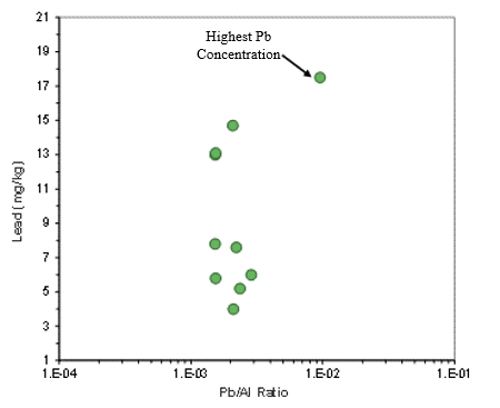
Figure 14‑12. Ratio plot of lead versus Pb/Al for background surface soil.
Source: Karen Thorbjornsen, APTIM.
14.7 Environmental Forensics Case Study—PAHs from Leaked Petroleum Versus Contaminated Fill
This site had various commercial and industrial uses since the 1800s, including a city dump, rail yard, and oil products terminal. The site is adjacent to a waterway whose shorelines progressed over many decades due to infilling of marshland associated with the site’s historic city dump. The oil terminal operated on only a portion of the site, wherein gasoline, kerosene, and diesel/fuel oil #2 (only) were off-loaded by barge, stored in aboveground tanks, and distributed by trucks from a loading rack. The rail yard was located at the terminus of a major railroad and operated from the mid-1800s until the 1960s.
Preliminary site assessments across the 13-acre site measured the concentrations of 16 priority pollutant PAHs (EPAPAH16) for 185 soil samples, which revealed regulatory exceedances of the cleanup standards in 74 soil samples at the site. Only 33 of these exceedances were due to 2- or 3-ring PAHs reasonably associated with gasoline, kerosene, or diesel/fuel oil #2; most exceedances were for high molecular weight, 4- to 6-ring PAHs in deeper soil intervals (>1 m). The study’s objective was to determine the sources of all PAHs detected in the soil samples, and specifically to distinguish PAHs derived from petroleum attributable to oil terminal operations (gasoline, kerosene, and diesel/fuel oil #2) versus nonpetroleum sources, potentially attributable to contaminated fill material and historical rail yard operations (for example, coal, coal ash, slag, and cinders).
Of the 185 soil samples, 108 were analyzed for TPH and PAH, the latter using the expanded list of PAH analytes that included 44 parent and alkylated PAHs and aromatic thiaarenes. The GC/FID chromatograms acquired using USEPA Method 8015 and PAH histograms acquired using modified USEPA Method 8270 revealed variable fingerprints for hydrocarbons and PAHs among the site’s soils, including apparent mixtures. The PAH concentrations were evaluated using PCA (Section 7.2.1), which yielded the factor score plot shown in Figure 14‑13. Three end-member sources of PAHs were recognized: pyrogenic fill, particulate coal, and light petroleum fuels. Based upon the PCA factor scores, many samples exhibited mixtures among these end-members.
Pyrogenic fill was dominated by 4- to 6-ring PAHs with homologues exhibiting a skewed pattern (Figure 14‑13), which is typical of pyrogenic sources (Section 7.3.1.2; Figure 7‑2; (Blumer 1976)). Soils containing particulate coal were recognized by a broad range of PAHs with bell-shaped homologue profiles typical of petrogenic sources (Figure 7‑2; (Blumer 1976)). However, because no such broad-boiling petroleum was handled at the site (only light fuels), this pattern was attributed to coal particles, not petroleum. This conclusion was supported by visual and microscopic examination of the soil samples. Finally, some soil samples exhibited a strong dominance of 2-ring PAHs attributed to weathered gasoline, while others exhibited 2- and 3-ring PAHs, along with sulfur-containing dibenzothiophenes, each exhibiting bell-shaped homologue profiles typical of petroleum, specifically, in this case, diesel/fuel oil #2 (Figure 14‑13).
Subsequent spatial analysis of the PCA-based results revealed that the soil samples identified as containing petroleum were mostly located proximal to former oil terminal operations (truck rack and pipelines). Those soil samples containing particulate coal were widely distributed on the site but were most common in the shallower soil intervals (<0.6 m). Finally, those soil samples containing pyrogenic fill also were widely distributed at the site, but these were found predominantly within deeper soil intervals (>1 m).
The chemical fingerprinting results, when interpreted in light of the site’s operational history, were used to constrain the spatial extent of soil at the site that was impacted by spilled petroleum attributable to the former oil terminal operations. Coal was attributed to historic rail yard operations wherein coal was stockpiled and used as a locomotive fuel. Its impact was limited to shallower soils. PAHs contained within the pyrogenic fill were found to be the dominant source of PAHs detected in the site’s soils and owing to the abundance of high molecular weight PAHs present in the fill (Figure 14‑13). These were largely driving the regulatory exceedances across the site and attributed to the infilling associated with the site’s historical dump operations.
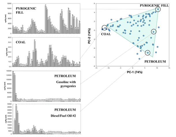
Principal component analysis (PCA) factor score plot (right) identifying three end-member PAH sources in the site soils, represented by PAH histograms (left). Note petroleum sources contain little 4- to 6-ring PAHs, which largely were responsible for regulatory exceedances at the site. Contaminated fill associated with historical landfilling resulted in an anthropogenic ambient background for this site.
Figure 14‑13. Principal component analysis (PCA) factor score plot.
Source: Stout (unpublished).

