11 Statistics
This section is intended to provide a general overview of the statistics used in establishing soil background values, comparing the site data to a background threshold value, or comparing site data to background data. The appropriate statistical approach will be influenced by the project goals and site-specific needs. Project stakeholders should identify and agree to an appropriate statistical approach when designing the soil background study. Many of the methods and procedures outlined in this section are discussed in greater detail elsewhere (for example, USEPA ProUCL Technical Guide (USEPA 2015)).
11.1 Data Requirements
11.1.1 Precautions
Data are essential in any scientific analysis, particularly statistical analysis. However, not all data are created equal and prior to any analysis, statistical or otherwise, the source and quality of data should be examined. Any conclusions are only as strong as the data used in the analysis. Therefore, it is essential to ensure data are not only of suitable quality, but also reflective of site-specific or regional conditions so that a representative background value is determined. Section 9 describes appropriate sampling methods and Section 10 describes appropriate laboratory methods, including data qualification. Further, many data quality issues are mitigated by developing a working conceptual site model (CSM) prior to any field sampling (ITRC 2013). As part of developing a CSM, DQOs can be developed that inform necessary quantity and quality of data (ITRC 2013). Developing a CSM and DQOs is discussed further in Section 8.
11.1.2 Appropriate use of statistics
Statistical analysis is a powerful technique that provides quantitative results to inform background and site decisions (ITRC 2013). Selection of the appropriate statistical analyses depends on the CSM, the study design, the sample design, and the data characteristics. Further, while statistical tests produce quantitative results, these results also have associated uncertainty. It is inherently infeasible to sample an entire volume of soil to obtain the exact background value; therefore, any statistically derived soil background value will also have inherent uncertainty. However, many statistical tests are calculated to a confidence level or interval, typically 95%, which provides some level of certainty. Statistical tests are sensitive to the confidence level or interval, which can produce false positive or false negative errors. Statistical background values, and these types of errors, are discussed in detail in Section 11.6. All statistical tests also have underlying assumptions. Violating these assumptions, or misapplying a statistical test, can produce erroneous and misleading results and degrade the defensibility of any decision at the site.
When applied appropriately, statistical methods provide quantitative results to define soil background concentrations and address project objectives (ITRC 2013). However, statistics are only one component of any scientific analysis. Statistics should not be used to compensate for low data quantity or poor data quality. Any scientifically defensible decision generally requires multiple lines of evidence in addition to statistical analyses (ITRC 2013). Additional examples of investigative methods include geochemical evaluation (Section 5) and environmental forensics (Section 7).
11.1.3 Minimum sample size
The appropriate application of statistics requires understanding the underlying assumptions and uncertainties of any statistical test, including the number of required samples. The appropriate sample size depends on the question being asked and the desired level of certainty. The minimum sample size is the number of individual samples required to conduct a specific statistical test or to calculate a specific statistical parameter with an acceptable level of uncertainty. Generally, a minimum sample size of 8–10 samples is required to do this ((USEPA 2009), (USEPA 2015)). This recommendation is applied in many state agency guidance documents ((IDEM 2012), (IDEQ 2014), (KDHE 2010)). However, depending on site characteristics and conditions or desired statistical power, more samples may be required. Some state agencies require a minimum sample size of 20 samples ((KEEC 2004), (MTDEQ 2005)), due to the typical heterogeneity of soils (MTDEQ 2005)).
In general, large datasets will provide better estimates of background concentrations and result in more powerful statistical tests (Cal DTSC 2008). However, the results of any statistical analysis are only as strong as the data. A strong dataset is a representative sample of the target population. A target population is the entire presence or distribution of a constituent in the soil (for example, arsenic concentrations in a soil type) (ITRC 2013). Generally, target populations cannot be fully characterized (ITRC 2013), as it is technically or financially infeasible to sample and analyze every segment of soil at a site. Therefore, each soil sample is only a small portion of the entire target population. A representative sample then is a dataset of soil samples that have statistical characteristics congruent with the statistical characteristics of the target population (ITRC 2013).
Therefore, a dataset must come from a representative sample of the target population, collected and analyzed using the appropriate methods discussed in Section 9 and Section 10. While a large dataset is desirable, nonrepresentative data (for example, collected using different sampling techniques or from a different target population) should not be included to arbitrarily increase the dataset size. Namely, a large dataset is not the same as a large dataset suitable for statistical analysis (ITRC 2013).
Ultimately, site conditions or characteristics and the chosen statistical test should inform the necessary number of samples. The statistical tests described in this section identify the minimum number of samples required, if appropriate. It is recommended that the appropriate regulatory agency also be consulted when determining the minimum number of samples ((IDEM 2012), (IDEQ 2014)).
11.1.4 Data selection
In addition to a minimum sample size, many statistical tests also have requirements regarding data selection or sampling. An underlying assumption of all statistics is that the collected measurements, or soil samples, are a random sample of the targeted population that is also free of any bias (IDEQ 2014). Random sampling is achieved through appropriate sampling techniques that are informed by the CSM. Random sampling does not necessarily imply that the entire soil at the site is sampled randomly, but that each target population is sampled randomly. Any investigative site will possibly contain several soil subgroups (for example, shallow or deep soils). Stratified sampling is the identification and sampling of each subgroup randomly. Section 9 of this document provides more discussion on appropriate sampling methods.
11.1.5 Target population
One key aspect of developing a CSM is determining the target population and whether the site includes one or more populations (ITRC 2013). A target population is the presence or distribution of a constituent in a soil (for example, arsenic concentrations in a soil type) (ITRC 2013). Target populations may be specific to a site, different soil groups, or background conditions (natural or anthropogenic ambient). As discussed previously in this section, it is imperative that all data for any statistical analysis be representative of the target population. Analysis of nonrepresentative data could lead to erroneous results. For example, a background value calculated from a dataset containing several unrelated populations will result in an erroneous result. However, the presence of multiple populations does not necessarily indicate a nonrepresentative dataset, as some background scenarios may inherently contain more than one subpopulation (for example, a site with several anthropogenic sources of the same constituent). Regardless, prior to any statistical analysis, the dataset must be evaluated to ensure it is representative of only one target population.
Site characteristics such as geology, soil depth, or geochemistry may indicate differing soil populations. For instance, deep soils may be representative of natural background conditions, while shallow soils would be more representative of anthropogenic ambient background conditions. In addition, graphical displays such as a quantile-quantile plot (Q-Q plot) or histogram can be used to determine the presence of data from several populations (Section 11.4). While these methods can reveal multiple populations, the selection of target population data from multiple populations can be subjective, requiring multiple lines of evidence and professional judgment. For example, in some cases for practical reasons and based on professional judgment, multiple background subpopulations may be combined in a statistical analysis.
Graphical methods (for example, box plots) and statistical methods (for example, Student’s t-test) can be used to evaluate and confirm the presence of multiple populations. These methods are discussed further in Section 11.4. Geochemical evaluations and forensic methods, discussed in Section 5, Section 6, and Section 7, can also be used to discern multiple populations within the dataset.
11.1.6 Underlying assumptions
Dataset size and representativeness are not the only requirements when applying statistics. Fundamentally, all statistics rely on three assumptions:
- The sampled data represent a random sample of the target population that is free from bias.
- The sampled data are representative of the target population.
- Each sample is random and not influenced by other measurements (each sample is independent of the other samples (IDEQ 2014)).
Further, specific statistical methods may have individual assumptions. For instance, some statistics have underlying assumptions regarding the distribution of the dataset (discussed in detail in Section 11.2). Prior to application of any statistical test, the assumptions of that method need to be understood.
11.2 Data Distribution
Data distribution is a descriptive statistic, often represented by a graphed curve, that describes all the values within a dataset and the frequency at which those values occur. Not all data are distributed in the same manner, and categories have been developed to describe common data distributions. Generally, statistical tests have underlying assumptions regarding sampling distribution. A prominent theorem in probability is the Central Limit Theorem, which states that the sampling distribution of the sample mean of a large number of independent random samples from a population is normal regardless of the distribution of the sampled population. Many common statistical methods rely on this theorem, and statistical tests that rely on distributional assumptions are referred to as parametric tests. However, in practice, environmental datasets may not have data distributions suitable for analysis using parametric methods. Therefore, prior to applying any statistical test, the data distribution must be understood. Applying a statistical test to a dataset that does not meet its distributional assumption will possibly produce erroneous and/or indefensible results (ITRC 2013).
The most recognized distribution is the normal distribution (Table 11‑1). The mathematical model of a normal distribution produces a smooth and symmetrical bell-shaped curve (ITRC 2013). The shape of the curve (or bell-shape) is determined by the mean and standard deviation of the dataset (ITRC 2013). The shape of the curve is directly related to the standard deviation; a small standard deviation produces a narrow distribution, while a larger standard deviation produces a wider distribution (ITRC 2013).
While a normal distribution is desirable for applying parametric statistics, many datasets have distributions that are not normal. Some common factors producing non-normal distributions include outliers and spatial or temporal changes (ITRC 2013). For example, natural background soil concentrations are often distributed asymmetrically (Chen, Hoogeweg, and Harris 2001) and are positively skewed (USEPA 2015).
While there could be additional considerations and guidance on the treatment of different data distributions, USEPA’s Statistical Program ProUCL considers two distributions that describe data with skewed distributions: lognormal and gamma (Table 11‑1; refer to USEPA’s ProUCL Technical Guide for in-depth discussion regarding theory and application of these distributions). Typically, skewed data are logarithmically transformed and tested for normality. If the transformed data distribution is normal, then the data was considered lognormal (IDEQ 2014). Traditionally, the log-transformed data were then analyzed using parametric statistical methods. However, the use of lognormal statistics can cause bias and unjustifiably elevated values for the mean and test statistics, especially for smaller datasets (<20–30 samples ((ITRC 2013), (USEPA 2015), (USEPA 2015), (Singh, Singh, and Iaci 2002)). Skewed data can also be described by the gamma distribution (Table 11‑1). The theory and application of the gamma distribution to skewed data were developed by Singh, Singh, and Iaci (2002) and incorporated into earlier versions of ProUCL. The application of the gamma distribution to skewed data and associated parametric methods is recommended in USEPA’s Unified Guidance, subsequent state agency guidance, and the current version of ProUCL ((USEPA 2009), (USEPA 2015), (USEPA 2015), (IDEQ 2014)).
Table 11‑1. Common distributions of environmental data
| Distribution Curve |
Basic Properties | Statistical Analysis Methods |
|
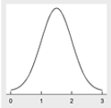 |
Normal | Data distribution is not skewed and centered around the mean | Analyze data set using parametric statistical methods |
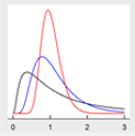 |
Lognormal | Data distribution is skewed and log transforming the data produces a normal distribution | Analyze data set using lognormal statistical methods only if data cannot be modeled by the normal or gamma distributions and the data set is not small (<15 – 20 samples) and highly skewed |
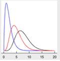 |
Gamma | Data distribution is skewed and modeled by the gamma distribution | Analyze data set using gamma statistical methods |
 |
Nonparametric | Data distribution cannot be modeled as a normal lognormal, or gamma distribution | Analyze data set using nonparametric statistical methods |
11.2.1 Parametric and nonparametric statistical methods
Parametric statistics can achieve high levels of confidence with a relatively small number of data points ((USEPA 2015), (USEPA 2015), (ITRC 2013)). However, environmental datasets often do not match the distributional assumptions for parametric methods, or the distribution cannot be determined because of insufficient sample size or a large number of nondetects (IDEQ 2014). In these instances, nonparametric methods may be more appropriate to use since they do not make distributional assumptions. Regardless, nonparametric methods still require a sufficient dataset and generally require larger datasets to achieve a similar level of confidence compared to parametric methods (ITRC 2013).
The first step in any statistical analysis is to determine the data distribution. Numerous methods are available that determine data distribution, typically by testing for normality. Normality can be examined graphically using normal probability plots or mathematical goodness of fit tests. Some common goodness of fit tests are listed below, including the distribution they can be used to test for ((USEPA 2015), (ITRC 2013)):
- coefficient of skewness and variation (normal and skewed distribution)
- Shapiro-Wilk test (normal distribution)
- Shapiro-Francia normality test (simplified version of Shapiro-Wilk for large, independent samples)
- Kolmogorov-Smirnov test (gamma distribution in USEPA’s ProUCL)
- Anderson-Darling test (gamma distribution in USEPA’s ProUCL)
Datasets determined to be normally distributed are generally analyzed using parametric methods. Parametric methods are the most appropriate for normally distributed data. Datasets with skewed distributions were traditionally analyzed using lognormal methods; logarithmically transformed data that resulted in a normal distribution were then analyzed using parametric methods. However, as discussed previously, Singh, Singh, and Iaci (2002) developed alternative methods using the gamma distribution that produce more accurate statistical results. Provided the dataset follows a gamma distribution, gamma statistical methods should be used to describe skewed datasets (USEPA 2015). USEPA’s ProUCL Technical Guide recommends that lognormal methods should be applied only if the dataset cannot be modeled by normal or gamma distributions and the dataset is not highly skewed and of small size (<15–20 data points). In general, if the data cannot be modeled by any distribution suitable for a parametric analysis (for example, normal, lognormal, gamma), or if the dataset is insufficient to determine the distribution, then the dataset is considered to follow a nonparametric distribution (Table 11‑1). If the dataset does not follow a distribution with available parametric methods, then nonparametric statistical methods should be applied (IDEQ 2014).
11.2.2 Uncertainties
As with any analysis, any determination of data distribution has uncertainties. Tests for normality depend on the values at the ends or tails of the ordered data, or the maximum and minimum values in the dataset (ITRC 2013). Therefore, numerous nondetects (more that 10% of the dataset) or outliers can affect normality tests. While nondetects and high concentrations may affect normality tests, these values may be typical and expected for a skewed environmental dataset that is truly not distributed normally. In general, several methods should be applied to determine data distribution, not just tests for normality. Goodness of fit tests can help identify the most reasonable distribution type, with statistical software providing the ability to easily test for several distributions and visually inspect the test results via Q-Q plots (see Section 11.4 for further discussion of graphic methods).
Additionally, large datasets collected over space or time can result in non-stationarity (data with a trend or changing variance). Specifically, soil samples collected over a large area for determining default soil background may include data that are not in the same distribution, causing the hypothesis of normality to be rejected by the distribution test even if the sample subsets are normally distributed (ITRC 2013). Trend tests or analysis of variance tests should be used if non-stationarity is suspected. Trend tests also rely on assumptions regarding data distribution; An analysis of variance test is a parametric test, and an equivalent nonparametric test is the Kruskal-Wallis test. In instances where non-stationarity is determined, additional analysis will likely be required, including release and transport evaluation, further sampling strategies, or different ways of combining and analyzing data (USEPA 2002). Additional analysis may be as simple as excluding a portion of the dataset that can be determined to be nonrepresentative or to be as complex as using a complex non-stationarity model to determine spatial sampling (Marchant et al. 2009)).
Making unverifiable assumptions regarding data distribution is not advisable (ITRC 2013), particularly regarding data normality. In instances where data distribution is not known, nonparametric methods should be used.
11.3 Treatment of Nondetects
Environmental datasets often contain “nondetect” results because of the limited sensitivity of laboratory methods to measure contaminants or because the analyte does not exist in soil (Figure 10‑1). This section is intended to cover what to do when the concentration of a given analyte in soil is below the detection limit (nondetect) and how to incorporate such data points in the statistical analysis. It is not intended to discuss laboratory analysis and results, which are discussed in Section 10. Specifically, Section 10.3 provides detailed discussion about detection and quantitation limits.
Nondetects in background datasets can complicate statistical analyses. There are several recommended procedures for treatment of nondetects. In general, nondetect results should be retained when using one of the appropriate methods described below. However, nondetects with detection limit (DL) values larger than the highest detected value in a dataset are usually excluded from further consideration to avoid ensuing complications in statistical analyses.
11.3.1 Substitution methods
Substitution or imputation methods replace nondetects with numerical values that are then treated as equivalent to detected values in statistical analyses. Typical substituted values include 0, various fractions of the DL, the full DL, or randomly assigned values between 0 and the DL. The most common form of imputation is ½ DL substitution, but there are also other proposed fractions of the DL such as DL/√2 (Antweiler 2015). Each of these alternatives is based on speculations or educated guesses about the shape of probability distribution functions of the nondetects. For example, ½ DL substitution assumes that the distribution of nondetects is symmetric between 0 and DL, while 1/√2 DL is based on the general assumption that the distribution of nondetects can be approximated by a right-triangular distribution with the DL as its mode and zero as its lower limit (see Figure 11‑1)
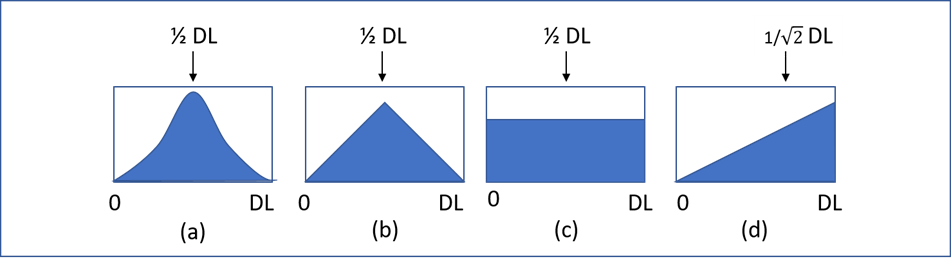
Symmetric distributions = (a), (b), and (c); right-triangular distribution = (d).
Figure 11‑1. Examples of assumed nondetect distributions and their corresponding substitution values.
Source: Leyla Shams, NewFields.
Most substitution methods are easy to understand and implement and, in some cases, produce results that are similar to certain more complex methods (for example, the median semi-variance (SemiV) method (Zoffoli et al. 2013)). In their extensive comparative evaluation of the performance of several methods for analyzing simulated censored datasets, Hewett and Ganser (2007) recognized the importance of ease of calculation/accessibility in dealing with datasets that include nondetects. Hewett and Ganser (2007) indicated that substitution methods are expedient and reasonably accurate, especially when dealing with datasets with small proportions of nondetects. However, substitution methods produce biased low estimates of population variance (Hewett and Ganser 2007). Such results can affect the reliability of certain statistics, including the estimates of the upper and lower confidence limits that rely on variance. For example, as discussed in ITRC (2013), using ½ DL substitution artificially reduces the variance of concentration data, resulting in a confidence interval that is smaller than expected.
In 2006, USEPA guidance supported the use of 0, ½ DL, or DL substitution in datasets with less than 15% nondetects (USEPA 2006). USEPA’s 2015 ProUCL Technical Guide restricted the use of ½ DL substitution only to datasets that are mildly skewed with less than 5% nondetects (USEPA 2015). Some investigators ((Hornung and Reed 1990), (She 1997), (Antweiler and Taylor 2008)) report the performance of ½ DL as being reasonable.
11.3.2 Kaplan-Meier method
The Kaplan-Meier (KM) method (Kaplan and Meier, 1958) is a nonparametric approach for construction of the cumulative distribution function of a dataset that contains censored data. The constructed CDF in turn is used to estimate the summary statistics of interest. The KM method sorts the dataset by detected and DL values ascendingly and relies on the number of records at and below each detected value to compute its cumulative probability.
The application of the KM method to environmental studies is relatively recent, when algorithms were developed to reformulate the method for left-censored environmental data (nondetects that are reported as less than the DL). Helsel (2005) proposed to transform censored data from left to right by subtracting each detected and DL value by a “large” number (also referred to as “flipping the data”), whereas Popovic et al. (2007) adjusted the algorithm formulas for left-censored data. This latter method has been adopted in USEPA ProUCL ((USEPA 2013), (USEPA 2015)).
KM does not require an assumption of data distribution or any substitution for nondetects, and thus can be applied to cases where the distribution of the data is not known or discernible ((Hewett and Ganser 2007), (USEPA 2015)), and is insensitive to outliers (Antweiler and Taylor 2008). KM results, however, are reliable only if the pattern of censoring is random and the probability of censoring is independent of DL values (Schmoyeri et al. 1996), (She 1997). This assumption means that the DL values associated with nondetects in a dataset must occur without displaying any preference to any particular range of concentrations. DL values in typical environmental datasets, however, are often associated with unique and/or low values that are lower than most, if not all, of the detected values. Older datasets with highly variable DLs may be more likely to meet the requirement of having a widespread distribution of DLs relative to measured values. In other words, nondetects are often concentrated along the lower end of the distribution. For such datasets, KM mean and upper confidence limit (UCL) results will be biased high.
Similar to other nondetect treatments, KM results become less reliable when the proportion of nondetects increases. PROPHET Stat Guide (Hayden et al. 1985) warned against the use of KM in cases of heavy censoring or small sample sizes. Helsel (2005) recommended use of the KM method on datasets with no more than 50% censored data, while ITRC (2013) recommended “no more than 50–70% nondetects.” Antweiler and Taylor (2008) recommended KM for summary statistics when datasets include less than 70% censored data.
KM has been promoted by many authors (including (Helsel 2005), (Antweiler and Taylor 2008), (USEPA 2015)), resulting in recommendations for its use within the environmental community. For example, (ITRC (2013), Section 5.7) recommended use of a “censored estimation technique to estimate sample statistics such as the KM method for calculating a UCL on the mean.” Hewett and Ganser (2007) tested KM against substitution, MLE, and regression on order statistics and found that KM “did not perform well for either the 95th percentile or mean.”
11.3.3 Regression on order statistics (ROS)
ROS is a semiparametric imputation technique (Helsel and Cohn 1988). To apply ROS, the results are sorted in an ascending order in accordance with their detected or DL values, as applicable. This step is followed by producing a plot of observed versus theoretical quantiles, sometime referred to as the Q-Q plot. Among the plotted quantiles, those associated with detected values are then subjected to linear regression. Each nondetect is then substituted with the predicted values based on the interpolated or extrapolated regression line using the order of their corresponding DL values ((Helsel 2005), page 68). A pictorial example is provided in Figure 11‑2.
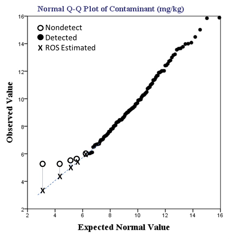
Figure 11‑2. ROS application example.
Source: Leyla Shams, NewFields (Generated by IBM SPSS Version 23 plus added graphics).
ROS can be applied to cases where statistical testing has confirmed that the measured data are derived from single populations. ROS is especially suitable for cases with 15–50% nondetects with either one or multiple detection limits ((ITRC 2013), (Sinha, Lambert, and Trumbull 2006)). However, ROS requires an a priori assumption about the distribution of the censored values: in particular, typical ROS applications assume that the distribution of the investigated data are approximately normal or lognormal (ITRC 2013). If the type of distribution is incorrectly assumed, the resulting ROS estimates (for mean, standard deviation, UCL, and upper tolerance limit (UTL) values) could be inaccurate. The presence of outliers can also distort the regression estimates of slope and intercept that are used to impute values for nondetects (USEPA 2015).
Hewett and Ganser (2007) found that overall, the log-probit regression-based methods “performed well across all scenarios.” Overall, ROS is most applicable to datasets that are derived from single populations, have limited skew, lack outliers, and have <50% nondetects (USEPA 2015). Datasets with 50% or more nondetects should not be subjected to ROS calculations ((ITRC 2013), (USEPA 2015)). ITRC (2013) further recommended that the approach should be applied with datasets representing at least eight to ten detected measurements, while USEPA (2015) recommended a minimum of four to six detected measurements.
11.3.4 Maximum likelihood estimation (MLE)
Maximum likelihood estimation refers to a family of parametric methods that, in essence, estimate parameters of assumed distributions by maximizing the likelihood of the occurrence of the actual detected and nondetect values in the dataset. (Helsel (2005), page 13) stated, “MLE uses three pieces of information to perform computations: a) numerical values above detection limits, b) the proportion of data below each detection limit, and c) the mathematical formula of an assumed distribution. Parameters are computed that best match a fitted distribution to the observed values above each detection limit and to the percentage of data below each limit.” The MLE-estimated distribution parameters are then used to calculate the summary statistics of the investigated data.
MLE can be used under a variety of assumed symmetric and asymmetric distributions. The vast majority of MLE applications in the literature have been developed for normal or lognormal distributions, which in some instances may reasonably match observed distribution of background datasets ((Akritas, Ruscitti, and Patil 1994), (Nysen et al. 2015)). Recent articles offer MLE solutions based on new classes of mixed distributions, which can be more representative of typical environmental datasets (Li et al. 2013)).
The primary cases where MLE is applicable are those in which the sample distribution can be reliably determined ((Helsel 2005), (ITRC 2013)). These are often datasets, derived from single populations, with larger sample sizes and/or a small proportion of nondetects (for example, less than 15% nondetects) (USEPA 2006). ITRC (2013), for example, recommended applying MLE to sample sizes of 50 or above and a detection frequency of more than 50%. If the type of underlying distribution is incorrectly assumed or cannot be identified, the resulting MLE estimates could be misleading.
Similar to datasets with nondetects, when applying MLE on censored datasets to compute upper limits such as UCLs and UTLs (see Section 11.6), the use of lognormal distribution should be avoided (Singh, Singh, and Me 1997). Despite its prevalence in environmental applications, assuming a lognormal distribution may lead to unrealistically elevated UCLs and UTLs, especially when the dataset is highly skewed. This issue has been illustrated throughout the ProUCL Technical Guide (97).
The most recent versions of USEPA’s ProUCL program have excluded parametric MLE methods, which USEPA (2015) described as “poor performing,” likely due to difficulties in verifying the distribution of left-censored datasets with multiple detection limits. In contrast, Hewett and Ganser (2007) found MLE methods in general to be strong performers when calculating the mean and 95th percentile values for data with known distributions.
11.3.5 Summary of nondetect treatment
The choice of the treatment of nondetects is driven by many factors that may require testing multiple procedures before identifying the appropriate method. Some practical rules for selecting an appropriate method for treatment of nondetects include:
- Substitution, such as 0, ½ DL, or DL, may be used, while recognizing that these methods often yield underestimated standard deviations, as discussed in Section 11.3.1.
- The Kaplan-Meier (KM) method has the advantage of being a nonparametric procedure, as discussed in Section 11.3.2. However, if DLs associated with nondetects are mostly below detected values, the KM mean and UCL would be biased high.
- Regression on order statistics (ROS) is ideal if the distribution of the detected values is clearly evident, as discussed in Section 11.3.3.
- MLE is ideal for datasets for which a reliable distributional assumption can be made, as discussed in Section 11.3.4.
- In cases where the dataset does not meet the above conditions for KM, ROS, or MLE, substitution may be used, while recognizing that these methods often yield underestimated standard deviations, as discussed in Section 11.3.1.
11.4 Graphical displays
Graphical displays of data can provide additional insight about a dataset that would not necessarily be revealed by using test statistics or estimates of confidence limits. These displays can be helpful in visualizing differences in means, variance, and distributions of background and site concentrations. Several graphing techniques that are commonly used include Q-Q plots, histograms, box plots, probability plots, and percentile plots. These are described in more detail below.
11.4.1 Quantile-quantile plot (Q-Q plot)
A Q-Q plot is a type of probability scatter plot generated by displaying data quantiles versus the theoretical quantiles of the specified distribution, including normal, gamma, and lognormal distribution. Departures from the linear display of the Q-Q plot suggest that the data do not follow the specified distribution. Note that theoretical quantiles are generated using the specified distribution. The correlation coefficient based upon the Q-Q plot is not a good measure to determine the data distribution. Statisticians have developed goodness of fit tests to determine data distribution. ProUCL has goodness of fit tests for normal, lognormal, and gamma distributions. Example Q-Q plots are shown in Figure 11‑3 and Figure 11‑4. If the background and site concentrations were very similar (Figure 11‑3), the two best fit lines would lie nearly on top of one another. If the concentration of contaminants at the site diverged from the background concentrations, the lines would diverge as shown in Figure 11‑4. Q-Q plots can also be used to compare a set of data against a specific distribution in a method called a theoretical quantile-quantile plot.
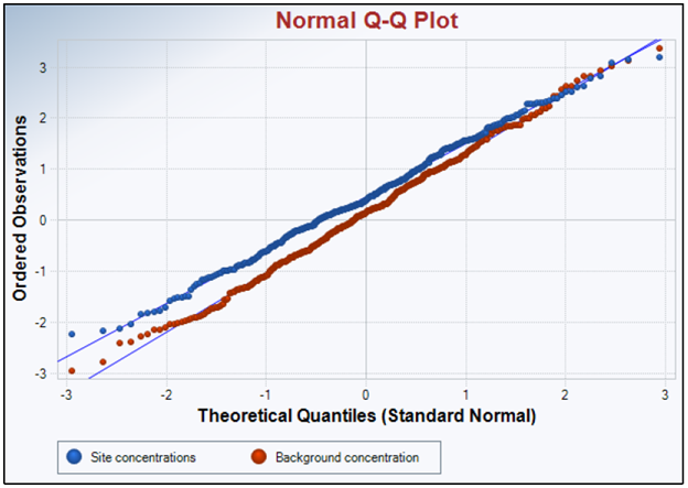
Figure 11‑3. Example Q-Q plot—Similar site concentration and background concentration.
Source: Jennifer Weidhaas, University of Utah (Generated by USEPA ProUCL version 5.1).
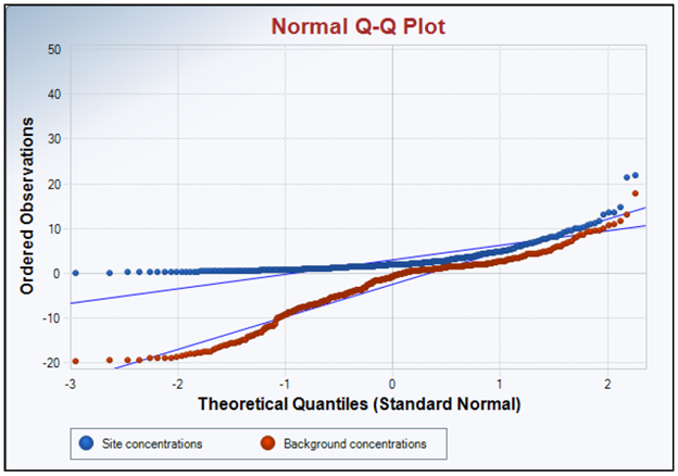
Figure 11‑4. Example Q-Q plot—Site concentrations diverging from background concentrations.
Source: Jennifer Weidhaas, University of Utah (Generated by USEPA ProUCL version 5.1).
The combined background and site Q-Q plot with highlighted background data can be used to identify the subpopulations associated with the background and to extract background data from the site data (ASTM E3242-20 (ASTM 2020)). However, the identification of exact break points (or threshold values for different populations) in a Q-Q plot is subjective and requires expertise for accurate evaluation. Guidance on these issues is provided in Section 3 of this document.
11.4.2 Histogram
Histograms are used to display continuous data and to graphically summarize the distribution of the dataset. These histograms can be used to compare the size and shape of the observed data and the potential skewness of the distribution. A histogram showing a lognormally distributed dataset is provided in Figure 11‑5 and a histogram showing a normally distributed dataset is provided in Figure 11‑6.
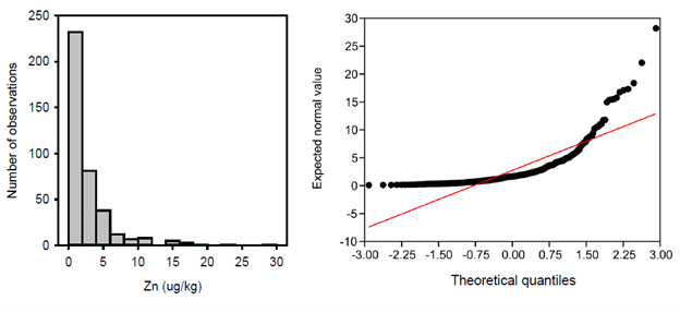
Figure 11‑5. Example histogram—Lognormal distributed data versus Q-Q frequency plot.
Source: Jennifer Weidhaas, University of Utah (Generated by Sigma Plot v 14.5).
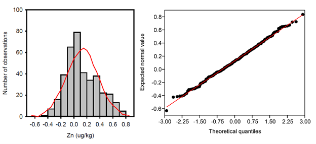
Figure 11‑6. Example histogram—Normal distributed data versus Q-Q frequency plot.
Source: Jennifer Weidhaas, University of Utah (Generated by Sigma Plot v 14.5).
The utility of histograms is limited if too few data points or samples are available, the proximity between the population means is too close, or there are unequal standard deviations for the populations. Histogram interpretation can be influenced by the number of bins included in the analysis. If too few bins are used, the shape is lost; conversely, if too many bins are used the shape can be lost as well. However, the histogram can be used to illustrate the conclusions drawn from the Q-Q plot and any outlier tests.
11.4.3 Box plot
Box plots summarize and display the distribution of a set of continuous data, such as the range of metal concentrations in soils at a site. These plots typically highlight five key points of the data: the median, the first and third quartiles (25th and 75th percentile values), and the minimum and maximum. Typically, values that are more than 1.5 times the interquartile range (the 75th percentile value minus the 25th percentile value) are considered outliers. Box plots are valuable as they can be quickly scanned to show the central tendency, range, and presence of outliers. Figure 11‑7 illustrates a box plot and depicts the interquartile range. When two box plots are shown side by side it is easy to make comparisons between datasets. Figure 11‑8 shows an example comparison of the range of metal concentrations in soils at two sites as depicted in box plots.
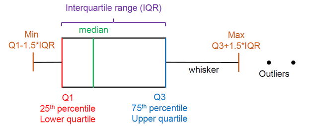
Figure 11‑7. Illustration of box plot and key characteristics.
Source: Jennifer Weidhaas, University of Utah.
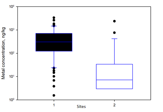
Figure 11‑8. Example comparison of the range of metal concentrations in soils at two sites.
Source: Jennifer Weidhaas, University of Utah (Generated by Sigma Plot v 14.5).
Box plots are typically most useful when datasets contain five or more values and nondetect values need to have a value assigned. Box plots are a quick, simple, and graphical method of displaying data. Further, they are easy to interpret and to compare two or more sets of data side by side. However, identification of outliers is fairly arbitrary and may not be conclusive. Identification of outliers in a box plot is user-defined, as it is possible to set the upper whisker at the maximum concentration, and the lower whisker at the minimum concentration. These plots are also limited in that they show only a single variable in each plot and cannot necessarily show relationships between variables or sites. Further, depending on how the data are plotted, all individual data points may not be shown. The box plot is not intended to be the only graphic used to evaluate site and background.
11.4.4 Probability plots
Probability plots are a graphical technique for assessing whether a dataset (for example, concentrations of a specific element) follows a given distribution (for example, normal or Gaussian distribution). The site data are plotted against a theoretical distribution so that if the data fit the distribution plotted, they fall along a straight line. The Q-Q plot is a type of probability plot (Figure 11‑5 and Figure 11‑6), namely the normal probability plot. Departures from the theoretical straight line indicate a departure from the specified normal distribution for the data. To determine the goodness of fit of the data to a distribution, the correlation coefficient is used. Typically, probability plots for several competing distributions are generated and the one with the highest correlation coefficient is likely the best choice.
11.4.5 Percentile plots
Percentile plots are nonparametric with concentration on the y-axis versus percentile on the x-axis (ASTM E3242-20 (ASTM 2020)). To construct these plots, first the concentration data are rank-ordered and then the corresponding percentile is applied to each concentration. An example of this kind of plot is provided in Figure 11‑9. Although no distributional assumptions are required, normally distributed data (if applicable) will appear as a straight line when a linear concentration scale is used. Lognormally distributed data (if applicable) will appear as a straight line when a logarithmic concentration scale is used (see Figure 11‑9). One application of percentile plots is in the identification of statistical outliers in a candidate background dataset. Such outliers will lie above or below the trend formed by the other data points. Breaks in slope may indicate bimodal or multimodal distributions or may indicate the presence of multiple samples with identical values. As with other graphical techniques, the data should always be inspected when evaluating the plots to identify the reasons for observed breaks in slopes and apparent outliers.
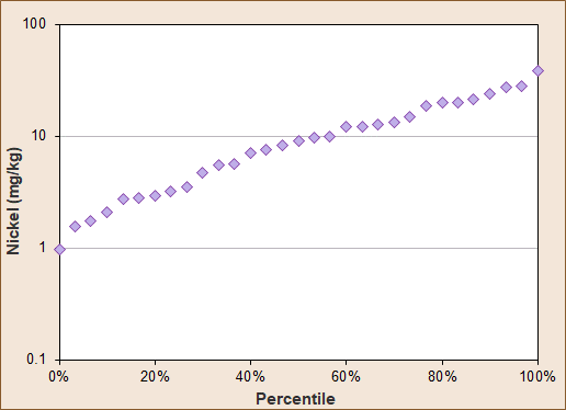
Figure 11‑9. Example percentile plot.
Source: Karen Thorbjornsen, APTIM.
11.5 Outliers
An outlier or an outlying observation refers to an extreme observation in either direction that appears to deviate markedly in value from other measurements of the dataset in which it appears. Outliers in environmental datasets can be classified into two broad groups (ASTM E178 2016 (ASTM 2016)):
- True outlier—“An outlying observation might be the result of gross deviation from prescribed experimental procedure or an error in calculating or recording the numerical value. When the experimenter is clearly aware that a deviation from prescribed experimental procedure has taken place, the resultant observation should be discarded, whether or not it agrees with the rest of the data and without recourse to statistical tests for outliers. If a reliable correction procedure is available, the observation may sometimes be corrected and retained.”
- False outlier—“An outlying observation might be merely an extreme manifestation of the random variability inherent in the data. If this is true, the value should be retained and processed in the same manner as the other observations in the sample. Transformation of data or using methods of data analysis designed for a non-normal distribution might be appropriate.”
USEPA (2006) stated that “failure to remove true outliers or the removal of false outliers both lead to a distortion of estimates of population parameters.” In practice, only outliers that are demonstrably erroneous or belonging to populations not representative of background conditions should be excluded from the background dataset. In background investigations, typical sources of error that can result in outliers include: (a) transcription error, (b) sampling error, (c) laboratory error, and (d) sampling of media not representative of background conditions as determined by forensic and geochemical analyses. In some cases, soil concentrations associated with known releases or isolated extreme values, such as the outlier displayed in Figure 11‑10, may be considered as not representative of background conditions. All other identified outliers should be retained and processed in the same manner as the other observations in the sample. A comprehensive review of outlier removal issues and recommended tests is presented in Grubbs (1969).
11.5.1 Graphical plots
Perceived high and/or low outliers can be visually identified using a probability plot. For this purpose, the measurements in the dataset are sorted in an ascending order and plotted against their corresponding cumulative probabilities, based on a specified distribution. The most common type of probability plot is constructed based in the normal distribution, hence referred to as the normal probability plot. Other forms of the probability plot include the Q-Q (quantile-quantile) plot and the P-P (probability-probability or percent-percent) plot. Normal Q-Q or PP plots can be used for any dataset regardless of their distribution. Log-normal probability plots are also used by practitioners, although USEPA (2015) warns against their use. Therefore, the use of log-normal probability plots is appropriate only if assessed and approved by a professional with statistical expertise.
A potential outlier may manifest itself as a high or a low value separated by a large gap from its preceding or ensuing ranked measurement, as displayed in Figure 11‑10. A gap is considered as “large” if it is visually much wider than the gaps displayed by other measurements in the probability plot. Authors, including van der Loo (2010), have proposed parametric procedures to analyze probability plot results to determine outliers.
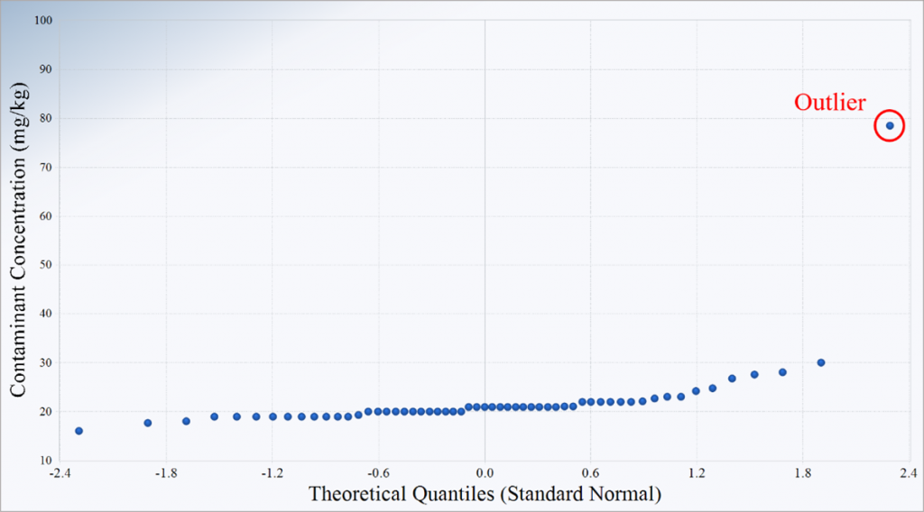
Figure 11‑10. Outlier in a Q-Q plot.
Source: Leyla Shams, NewFields (Plot generated by USEPA ProUCL 5.1 (USEPA 2015)).
11.5.2 Statistical tests
There are well-established procedures to test for statistical outliers. Each statistical test requires a pre-identified number of perceived high and/or low outliers and an assumed distribution of the background population. Typical occurrences include a single outlier, or two or more outliers on the same or opposite sides of the dataset.
As listed in Table 11‑2, common statistical outlier tests, including those presented in ASTM E178-16a (ASTM 2016), assume the normality or symmetry of the measurements after the removal of outliers. As noted in ASTM E3242-20 (ASTM 2020), for many environmental datasets, the normality assumption is incorrect, which can lead to erroneous outlier identifications. This problem is further exacerbated when the above statistical tests are applied repeatedly, through the iterative removal of perceived outliers. Under such procedures, shrinking standard deviations caused by continuous exclusion of perceived outliers produces an increasing likelihood of incorrect identification of additional outliers. The result is the calculation of biased, unrepresentative results from an incorrectly truncated dataset. In many instances, graphical techniques, such as normal Q-Q plots or box plots, may be more appropriate for identifying outliers. In these cases, a normal Q-Q plot (on untransformed data) may be used as an exploratory tool to identify outliers, and not to determine normality of data (Hoaglin, Mosteller, and Tukey 1983).
Table 11‑2. Outlier tests
Source: Developed from (USDON 2002), Table B-3, and ASTM E3242-20 (ASTM 2020), Table X4.1.
| Statistical Test | Assumptions | Advantages | Disadvantages |
| Dixon’s test |
|
|
|
| Discordance test |
|
|
|
| Rosner’s test |
|
|
|
| Walsh’s test |
|
|
|
The above outlier tests are commonly cited in environmental guidance documents and were developed when environmental datasets were small and the computing power was limited. Newer outlier identification methods that include robust methods are available, such as Hoaglin, Mosteller, and Tukey (1983), Rousseeuw and Leroy (1987), Rousseeuw and Zomeren (1990), Iglewicz and Hoaglin (1993), Maronna, Martin, and Yohai (2006), Singh and Nocerino (1995), and Singh (1996). Several effective and robust outlier tests are available in the commercial software packages, including SAS and STRATA.
11.6 Confidence Interval Limit, Coefficient, and Limit
A confidence interval is a range having an upper limit value and lower limit value. The true value of the parameter of interest lies within this range/interval. The confidence interval is determined based on the dataset that has been sampled and is only as accurate as the data one has obtained. A confidence interval places a lower limit or an upper limit on the value of a parameter, such as soil metal concentrations.
A confidence coefficient displays how confident the user is the true value will be within the confidence interval. In other words, how much confidence there is that the true value of the parameter of interest does indeed lie between the upper and lower limits of the confidence interval. It is generally recommended that a confidence coefficient of 95% be used, meaning there is a 95% chance that the true value lies between the upper and lower confidence interval values. Confidence coefficients are expressed as values between 0 and 1. A 95% confidence coefficient is expressed as 0.95.
A confidence limit is the lower or upper boundary of a confidence interval (the range of possible values that includes the true value of the parameter of interest). For risk assessment we are usually interested in the upper boundary since we need to be reasonably conservative to ensure we are being protective. When we are choosing an exposure concentration, we usually choose the upper confidence limit of the mean since this gives us a reasonably conservative estimate of what the true mean might be. When we are establishing soil background values (BTVs) we also usually consider using the upper confidence limit of the range of background concentrations to be reasonable to compare to the site concentrations. It is important to carefully consider what site concentrations will be used to compare to this upper confidence limit of soil background to ensure we are being reasonably protective, as discussed in Section 3.
11.7 Statistical Values Used to Represent Background
Although soil background is properly expressed as a range of values, regulators generally need to express it as one single value to be able to use it in risk assessment. Often, for this purpose regulators use soil background threshold values or BTVs. BTV is defined as a measure of the upper threshold of a representative background population, such that only a small portion of background concentrations exceed the threshold value. BTVs are usually used for site delineation purposes, or point-by-point comparison to individual site data to identify localized contamination ((Geiselbrecht et al. 2019), ASTM E3242-20 (ASTM 2020)). Appendix A contains additional information on upper limits commonly used to represent background.
Regardless of the chosen BTV, point-by-point comparisons are prone to produce false positive errors. That is, as the number of comparisons increases, the chance of incorrectly concluding at least one erroneous above-background exceedance approaches 100%, even when the site data are within background ranges (Gibbons 1994). As stated in ASTM D6312-17 (ASTM 2017), “Even if the false positive rate for a single [comparison] is small (for example, 1 %), the possibility of failing at least one test on any [site dataset] is virtually guaranteed.” Due to this limitation, caution should be used when conducting point-by-point comparisons. The U.S. Department of the Navy (USDON 2003) recommended against point-by-point comparisons, except when coupled with reverification sampling ((Gibbons 1994), ASTM D6312-17 (ASTM 2017)). In practice, point-by-point comparisons to BTV are very useful and efficient screening procedures. If exceedances above BTV are detected, then more robust site-to-background tests can be conducted to determine presence or absence of concentrations above background conditions.
Applications of BTV yield reliable results only if the representative background dataset contains an adequate number of measurements. Adequacy of the background sample size is dependent on the intended application, assumptions about the underlying distribution of the chemical concentrations, and the tolerable error rates. These error rates include falsely declaring a site clean (false negative) and falsely declaring a site contaminated (false positive). Falsely declaring a site clean is often of more concern to regulators, and the error rate is set at 5% by convention. The total sum of error rates should not exceed 25% (Gibbons 1994). As a result, the rate of falsely declaring a site contaminated is often set at a value less than or equal to 20%. Inadequate background sample sizes can lead to unreliable or inappropriate conclusions. A more comprehensive review of this topic and the associated literature is presented by Cochran (1997).
Values commonly used to represent BTVs include the upper percentile, the upper prediction limit (UPL), the upper tolerance limit (UTL), and the upper simultaneous limit (USL). A summary of these values is presented in Table 11‑3. (USEPA (2015), Section 3) provides detailed discussions and recommendations about the applications of these BTVs. For metals, natural exceedances of BTVs are common and can be verified through geochemical evaluation (Section 5). These exceedances are expected because trace element concentrations naturally span wide ranges, and their distributions are typically right skewed; it is difficult for any background dataset to fully capture these ranges of concentrations.
Table 11‑3. Summary of values used to represent BTV
| Value | Acronym | Description |
| Upper percentile | Not applicable | Value below which a specified percentage of observed background concentrations would fall |
| Upper confidence limit | UCL | Upper limit of 95% confidence interval |
| Upper prediction limit | UPL | The value below which a specified number of future independent measurements (k) will fall, with a specified confidence level |
| Upper tolerance limit | UTL | The UCL of an upper percentile of the observed values |
| Upper simultaneous limit | USL | Value below which the largest value of background observations falls with a specified level of confidence |
11.7.1 Upper percentile
An upper percentile is the value below which a specified percentage of observed background concentrations would fall. For example, the 95th percentile is the value below which 95% of observations may be found. Upper percentiles, when used for point-by-point comparison, can yield excessive false positive rates approaching 100%, which are exacerbated when dealing with small background datasets or background datasets consisting of multiple subpopulations.
Estimates of upper percentiles are reliable (not prone to over- or underestimation) if the background dataset is adequately large and representative of a single population. As noted in (USEPA (1989), Section 4.6.1, p. 4–17), the adequacy of the number of measurements depends on statistical and practical considerations. For example, when calculating a nonparametric BTV, if the risk assessor wants to be 90% confident that at least one of the measurements falls within the upper 5th percentile of the background population, then 45 measurements are needed, (90% = 1 – (1 – .05)45). If for practical reasons, only 27 background samples are collected, the resulting confidence would be 75%, (75% = 1 – (1 – .05)27). This example illustrates that the adequate number of measurements is driven by statistical and practical considerations. Other confidence limits are shown in Table 11‑4 and calculated using the following equation:
Upper confidence limit = [1 – (1 – (upper percentile needed)number of samples)]*100
When planning a background sampling event, the assistance of a professional with statistical expertise is recommended.
Table 11‑4. Relationship between number of samples tested and the resulting UCL for an upper 5th percentile of the background population
| Number of Samples Tested | UCL | UCL Calculation |
| 10 | 40% | [1-(1-0.05)^10)]*100=40% |
| 20 | 64% | [1-(1-0.05)^20)]*100=64% |
| 30 | 79% | [1-(1-0.05)^30)]*100=79% |
| 40 | 87% | [1-(1-0.05)^40)]*100=87% |
| 50 | 92% | [1-(1-0.05)^50)]*100=92% |
| 60 | 95% | [1-(1-0.05)^60)]*100=95% |
| 70 | 97% | [1-(1-0.05)^70)]*100=97% |
| 80 | 98% | [1-(1-0.05)^80)]*100=98% |
| 90 | 99% | [1-(1-0.05)^90)]*100=90% |
11.7.2 Upper confidence limit
The accuracy of any statistical estimate is often quantified by its confidence interval, which is the range of values around the estimate that contains, with certain probability (for example, 95%), the true value of that estimate. The upper limit of this interval is referred to as the upper confidence limit or UCL. The UCL of the mean is the common measure of point exposure concentration in risk assessments. However, since the mean is a measure of the central tendency of a dataset, UCL of the mean should not, under all but select circumstances, be used as a BTV because the result would be excessive false positive results.
11.7.3 Upper prediction limit
The UPL is the value below which a specified number of future independent measurements (k) will fall, with a specified confidence level. For example, the 95% UPL of a single observation (k=1) is the concentration that theoretically will not be exceeded in a new or future measured background concentration with a 95% confidence level. Similar to the upper percentile, the use of UPL based on small background datasets (<50 measurements) with multiple subpopulations for point-by-point comparisons can lead to excessive false positive error rates. If the UPL is calculated based on only one future measurement (k = 1) but more (>1) future measurements are obtained, then the resulting UPL will be unrealistically conservative, and the false positive error rate will be even higher.
11.7.4 Upper tolerance limit (UTL)
The UTL is the UCL of an upper percentile of the observed values. A UTL is designated by its confidence and coverage. Coverage defines the targeted upper percentile estimate (for example, 95% coverage implies that the targeted upper percentile is the 95th percentile). Confidence, on the other hand, is related to the interval in which the true value of the upper percentile should occur. For example, the 99-95 UTL represents the 95% upper confidence level (95% UCL) of the 99th percentile value. This means that 95% of future sampling events generate 99th percentiles that will be less than or equal to 99-95 UTL.
When conducting point-by-point comparisons using the UTL, the false positive error rates stay the same, irrespective of the number of comparisons (USEPA 2015). The 95-95 UTL has become the most common measure of BTV in practice. However, when dealing with site datasets with numerous measurements, even a reasonable false positive error rate would yield a number of erroneous above-background classifications; this needs to be taken into account when interpreting the data.
11.7.5 Upper simultaneous limit (USL)
The USL is the value below which the largest value of background observations falls with a specified level of confidence (USEPA 2015). USL is specifically used to mitigate the issue of excessive false positive error rate in point-by-point comparisons. However, due to the sensitivity of the USL to outliers, USEPA (2015) recommended its use only in background datasets devoid of outliers or multiple subpopulations.
11.8 Statistical Tests to Compare Site and Background Datasets
There are many statistical tests that can be used to compare a site dataset to a soil background dataset. The test that is most appropriate in each scenario will depend on the site-specific situation. Statistical tests that can be used are listed in the table below along with the associated advantages and disadvantages of each.
In practice, point-to-point comparisons of individual site data to the BTV are used for either delineation purposes or identifying localized contamination (Geiselbrecht et al. 2019). More comprehensive comparisons of site and background datasets involve the use of two-sample tests (USEPA 2006). As noted in USDON (2002), in contrast to point-to-point comparisons, two-sample tests are less prone to falsely identifying above-background conditions.
ASTM E3242-20 (ASTM 2020) provides a list of common two-sample tests used in environmental applications, as reproduced in Table 11‑5. Each test is based on a specific statistical hypothesis test. Some of these tests, such as the parametric t-test and the nonparametric Mann–Whitney U test, are geared toward the comparison of central tendencies of two datasets, to identify widespread contamination. Other tests focus on the comparison of the upper tails of the two datasets to identify localized contaminations (Geiselbrecht et al. 2019).
Table 11‑5. Assumptions, advantages, and disadvantages of common two-sample tests
Source: ASTM E3242-20 (ASTM 2020), Table X4.2.
| Test Statistic | Objectives/Assumptions | Advantages | Disadvantages |
| Quantile test |
|
|
|
| Wilcoxon rank sum (WRS) test also referred to as the “Wilcoxon-Mann-Whitney test” or “Mann Whitney U test”) |
|
|
|
| Gehan test |
|
|
|
| Tarone-Ware test |
|
|
|
| Student’s t-test |
|
|
|
| Satterthwaite or Welch’s two-sample t-test |
|
|
|
| Two-sample test of proportions |
|
|
|
| Levene’s test |
|
|
|
| Shapiro-Wilk test |
|
|
|
Reprinted, with permission, from ASTM E3242−20 Standard Guide for Determination of Representative Sediment Background, copyright ASTM International, 100 Barr Harbor Drive, West Conshohocken, PA 19428. A copy of the complete standard may be obtained from ASTM International, www.astm.org.
In many instances, both widespread contamination and localized contamination should be tested concurrently. Selection of the appropriate test is contingent on the specific conditions, including the target statistics of interest and the type of distributions displayed by the investigated site and background datasets, as well as their variance equivalency. Geiselbrecht et al. (2019) developed a decision flow diagram for selecting the appropriate types of tests, as reproduced in Figure 11‑11. In practice, nonparametric tests are often preferred because they do not require any specific distributional assumption about the investigated site and background data.
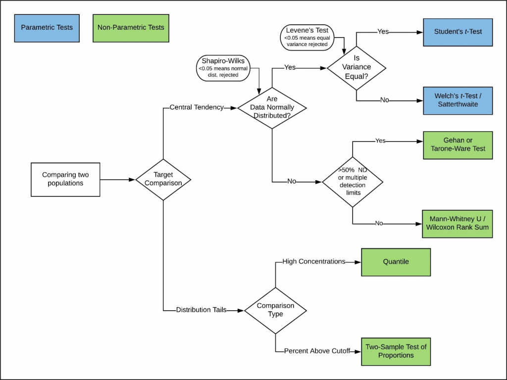
Figure 11‑11. Statistical tests for comparison of two datasets.
Source: Adapted from Geiselbrecht et al. (2019)
11.9 Statistical Software
There are many readily available software packages that can be useful for background data analysis (Table 11‑6). The following discusses some commonly used software but is far from comprehensive. Other software may be equally pertinent, such as ArcGIS or Visual Sample Plan for specific project needs, but this summary is meant only to make the reader aware of the existence of broadly useful statistical software and to highlight features that may be most useful for their situation.
While most of the statistical analysis programs listed below will have the capability to conduct many of the analytical methods required for background statistical analysis, not all programs will be able to easily conduct all methods. Choosing statistical software for the background analysis needs may have other considerations than simply cost or capabilities (for example, limited statistical experience or regulatory agency requirement).
Because software is subject to continual development, the statements made herein regarding specific software programs will become outdated over time. Future versions of programs described herein may feature expanded capabilities, whereas some programs that are currently popular may become less so in the future. Therefore, it is recommended that users research available software options periodically and treat the recommendations presented herein as general guidelines.
It is important that someone using statistical software packages understand the statistics behind the software and the uncertainties. Appropriate use of software requires valid data and someone with sufficient understanding of both statistics and the specific situation being evaluated to make reasonable professional judgment decisions using multiple lines of evidence (of which software statistical analysis would be only one). Decisions should never be made using the software analysis results alone without other lines of evidence.
Table 11‑6. Statistical software commonly used in computations involving background concentrations in risk assessments
| Software | Capability | Advantages | Disadvantages |
| USEPA ProUCL | Parametric and nonparametric two-sample tests Multiple options for parametric and nonparametric BTV calculations; options for distribution tests and datasets with nondetects Outlier identification tests Trend tests |
|
|
| Microsoft Excel | Point-by-point comparisons; parametric two-sample tests; limited graphical capabilities |
|
|
| R code | Open-source code offering a wide variety of statistical and data visualization tools, including all those offered by ProUCL |
|
|
| Python | Open-source code offering a wide variety of statistical and data visualization tools, including all those offered by ProUCL |
|
|
| Integrated Statistics Programs (for example, SAS, SPSS, Stata, Statistica, Minitab, MATLAB, Wolfram Mathematica) | Commercial packages offering a wide variety of statistical and data visualization tools, including all offered by ProUCL |
|
|
11.9.1 USEPA’s ProUCL
USEPA’s ProUCL software, currently version 5.1 released May 2016, includes a thorough user guide as well as a technical guide. Version 5.2 is under development and is poised to be released soon. The overwhelming majority of user functionality will be the same between the two versions. The user and technical guides have been updated for version 5,2 as well. The guides walk users through an extensive suite of statistical procedures, including two-sample hypothesis tests, trend analysis methods, BTV calculation, and UCL estimation. The BTV and UCL modules provide several different methods for calculating BTVs and UCLs of the mean. Additionally, there are multiple training presentations available for those just getting started or looking to master the use of ProUCL. Both the ProUCL software and the trainings can be found at USEPA’s ProUCL website.
USEPA and state regulatory agencies often use ProUCL because it is recommended by USEPA, it’s free and easy to use, and it provides a consistent way to regulate all parties fairly. State regulatory staff often do not have statisticians and do not always have time to learn statistics as thoroughly as they may like to. This software allows users without formal statistical training to obtain accurate results for common statistical procedures. The user interacts with the software via a graphical user interface (GUI) that does not require coding or statistical knowledge (Figure 11‑12). As stated earlier, it is important that one using this software understands the statistics being used and the uncertainties involved so they can make an informed decision based on multiple lines of evidence.
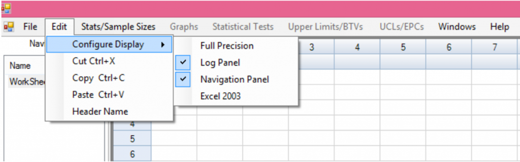
Figure 11‑12. Example USEPA ProUCL interface.
Source: (USEPA 2015).
Additionally, users can create graphical outputs, though these are limited to histograms, box plots, Q-Q plots, and trend analysis plots (Figure 11‑13). ProUCL does not handle other graphical outputs discussed in later sections, such as index plots, ratio plots, and bar plots.
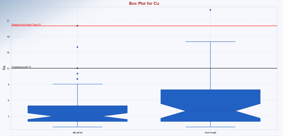
Figure 11‑13. Example USEPA ProUCL box plots.
Source: (USEPA 2015).
11.9.2 Microsoft Excel
Microsoft Excel is likely the most well-known software for data entry and tabular manipulation. This software comes with the backing of Microsoft and is directly integrated as part of the ProUCL software, as using Excel formats for input and output within ProUCL is standard. Within Excel itself, there are basic tools for data visualization, a free ExcelAnalysis Toolpak plugin, and a programming language (Visual Basic for Applications or VBA) to conduct more advanced analyses (“macros”) than those provided in Excel’s built-in functions. There is a limited free VBA version and a more robust paid version for both Windows and Mac OSX. There are also paid and free statistical analysis plugins for both Windows (for example, XLSTAT and Analyse-it) and Mac OS X (Real Statistics Using Excel). With this in mind, Excel was certainly not intended as a full-fledged background statistical analysis tool and is most suited to simple exploratory data analysis.
11.9.3 R
R is an open-source language and coding environment for statistical computing and graphics. Due to this classification as a language, as opposed to simply a software package, the background statistical analysis possibilities are basically limitless. If a user has the resources and know-how to create an analysis method for the problem in question, it can be tailored to virtually any site-specific problem or issue complexity level. R is also capable of producing all the same statistical analysis that can be achieved in ProUCL.
Because R is a coding language, it does require significantly more statistical understanding to use over USEPA’s ProUCL software. To help with this challenge, there are numerous packages available through R’s Comprehensive R Archive Network (CRAN). While those packages do not necessarily have any guarantees to their reliability, many are heavily used and regularly maintained by skilled statisticians. Additionally, all code used in building functions included in those packages is visible to R users should they desire to inspect the underlying code further.
One of the biggest advantages that R provides is its ability to produce high-quality graphical deliverables. In addition to the graphic capabilities that come with the core R software, freely available packages, such as ggplot2 and plotly, can provide customizable and interactive (plotly) graphical results. This can be taken a step further using R’s Shiny app suite, which allows for web hosting of interactive tools. This app suite allows those receiving the deliverable to visualize data or statistical results in flexible ways. Bearing all of that in mind, the background statistical analysis conducted within R is only as reliable as the individual or team that conducted the analysis, so careful quality control and assessment are advised.
R is free and is compatible with Microsoft Windows, Mac OS X, and Linux. Some existing packages within R may function only on a subset of these operating systems. R can be obtained from the R-Project website.
11.9.4 Python
Python is a freely available coding language capable of many of the same things as R. However, this language and its supporting packages tend to focus more on programming and integration with other software (for example, GIS) as opposed to the statistician-oriented approach within R. Python users have developed many freely available packages that provide for a widely customizable approach to statistical analysis. However, at the time this guide was written, there are significantly fewer purpose-built statistical analysis packages available for Python then there are for R.
11.9.5 Integrated statistical programs
There are many commercially available statistical software programs that effectively combine database, graphical, and statistical capabilities with a relatively accessible user interface. The key benefit of using such programs is that they are intuitive to use and can quickly generate decently attractive graphics and accurate analytical results based on a range of typical assumptions and inputs. The downsides of such programs can be lack of flexibility in graphics and analysis relative to programs such as R or Python, and relatively high cost considering most other presented options are free to the user. Integrated statistical programs also lack the focus of a program such as ProUCL, which includes functions specific to the analysis of environmental data. Examples of integrated statistical programs include, but are not limited to SAS, IBM SPSS, Stata, TIBCO Statistica, SYSTAT, MYSTAT, and Minitab. The most popular programs require payment to access, typically through an annual subscription service. GNU PSPP is a free program intended as an alternative to SPSS and similar programs. Currently, PSPP provides only a small number of statistical methods relative to SPSS or the other programs listed above.
While limited relative to R or Python, the integrated statistical programs noted above have sufficient capabilities to support the estimation of background conditions or to compare site conditions to background. These capabilities include summary statistic calculation, hypothesis testing tools (for example, t-test and Wilcoxon Rank Sum test), graphical comparison tools, and other tools, depending on the specific program. For background analysis, integrated statistical programs may be more advanced than necessary; the statistical methods and graphics capabilities in ProUCL or potentially less expensive software, such as Excel add-ins like XLStat, or data visualization programs like SigmaPlot, may be sufficient to characterize soil background conditions.

